intro to biostatistics and data variables (2).ppt

CONTENTS
 Introduction
 What is statistics?
 Biostatistics
 Uses of Biostatistics
 Data
 Sample & Sampling designs
 Probability
 Statistical Significance (Tests of significance )
 Correlation & Regression
 Conclusion
 References

“ when u can measure what you are
speaking about and express it in
numbers, you know something about it ;
but when you cannot express it in
numbers , your knowledge is of meagre
and unsatisfactory kind.”
- Lord Kelvin

‘Statistic’ or ‘Datum’ – in singular, it is measured
or counted fact or piece of information stated as
figure.
‘Statistics’ or ‘Data’ – Plural of the same , stated
in more than one figures.
Statistic -Statista (Italian word)- Statesman
Statistik ( German word )–political state
John Graunt (1620-1674) - Father of health statistics

Definition
Statistics:
Principles and methods for collection,
presentation, analysis and interpretation of
numerical data.
Biostatistics:
Tool of statistics applied to the data that is
derived from biological science.

Why need biostatistics ?
 Define normalcy
 Test the difference b/w two population
 Study the correlation or association b/w
two or more attributes
 To evaluate the efficacy of vaccines, sera
etc by control studies
 Locate , define & measure extent of
disease
 Evaluate achievements
 Fix priorities

The five fundamental processes involved
in organization of oral health care services.
1. Acquisition of information.
2. Dissemination of information.
3. Application of knowledge and skill.
4. Judgement or evaluation.
5. Administration.

Uses of biostatistics in Public Health Dentistry
 Assess the state of oral health in community
 Indicate basic factors underlying state of oral
health
 Determine success or failure of specific oral
health care programmes or to evaluate the
programme action
 Promote health legislation and in creating
administrative standards for oral health

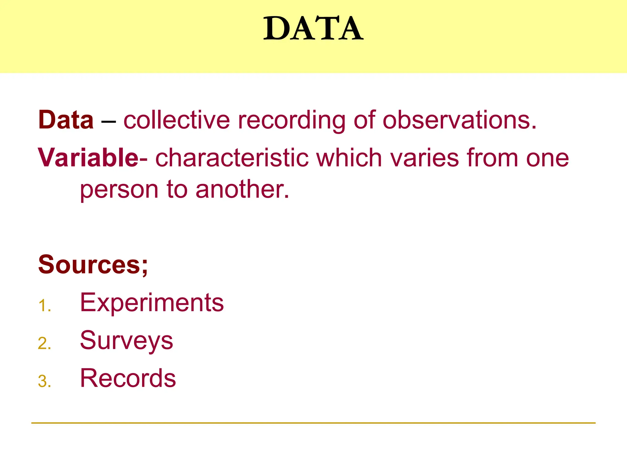
DATA
Data – collective recording of observations.
Variable- characteristic which varies from one
person to another.
Sources;
1. Experiments
2. Surveys
3. Records

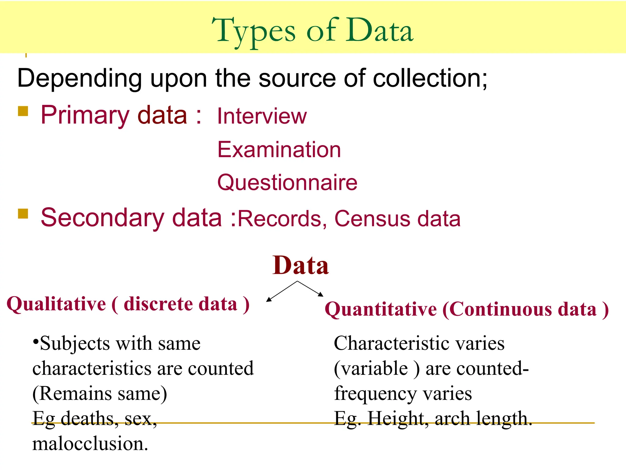
Types of Data
Depending upon the source of collection;
 Primary data : Interview
Examination
Questionnaire
 Secondary data :Records, Census data
Data
Qualitative ( discrete data ) Quantitative (Continuous data )
•Subjects with same
characteristics are counted
(Remains same)
Eg deaths, sex,
malocclusion.
Characteristic varies
(variable ) are counted-
frequency varies
Eg. Height, arch length.

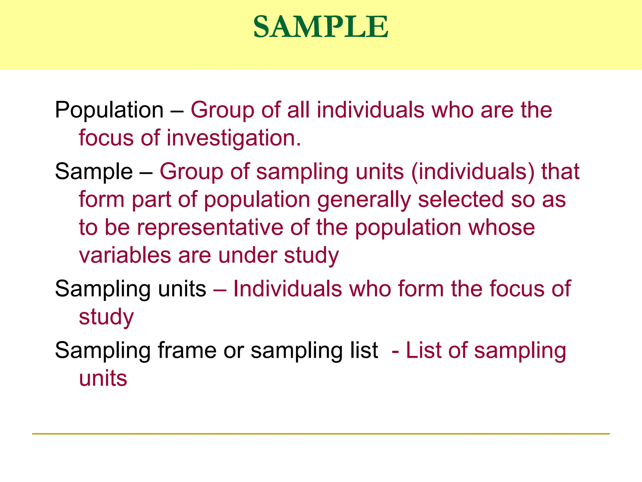
SAMPLE
Population – Group of all individuals who are the
focus of investigation.
Sample – Group of sampling units (individuals) that
form part of population generally selected so as
to be representative of the population whose
variables are under study
Sampling units – Individuals who form the focus of
study
Sampling frame or sampling list - List of sampling
units

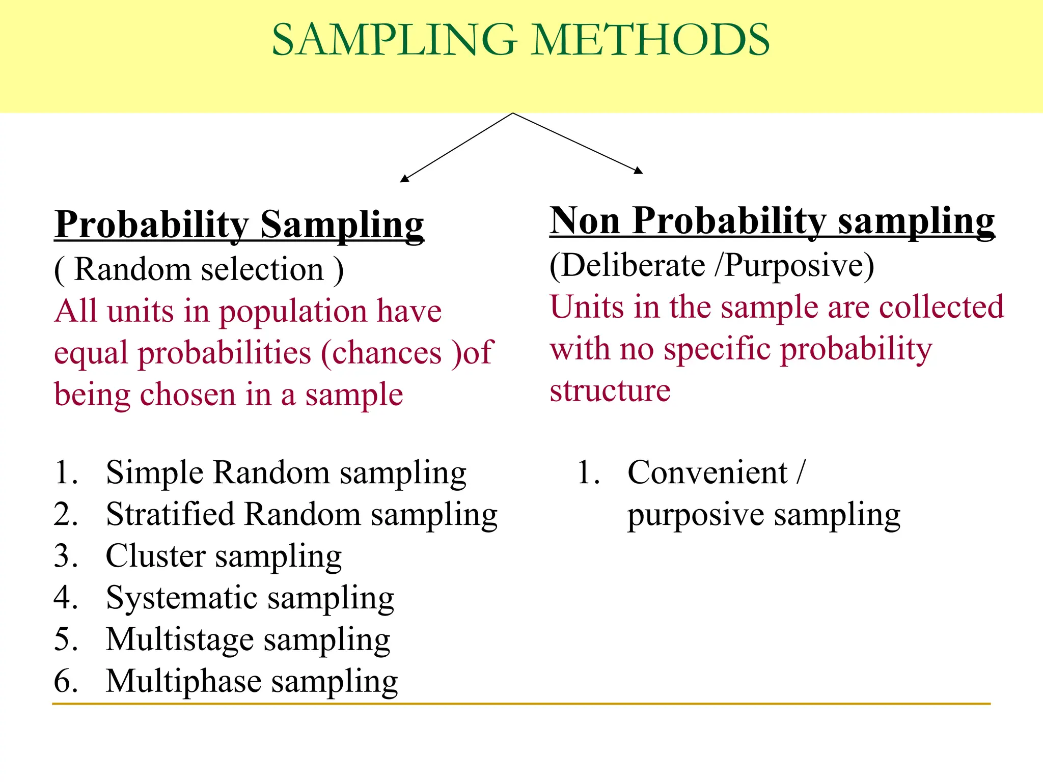
SAMPLING METHODS
Probability Sampling
( Random selection )
All units in population have
equal probabilities (chances )of
being chosen in a sample
Non Probability sampling
(Deliberate /Purposive)
Units in the sample are collected
with no specific probability
structure
1. Simple Random sampling
2. Stratified Random sampling
3. Cluster sampling
4. Systematic sampling
5. Multistage sampling
6. Multiphase sampling
1. Convenient /
purposive sampling

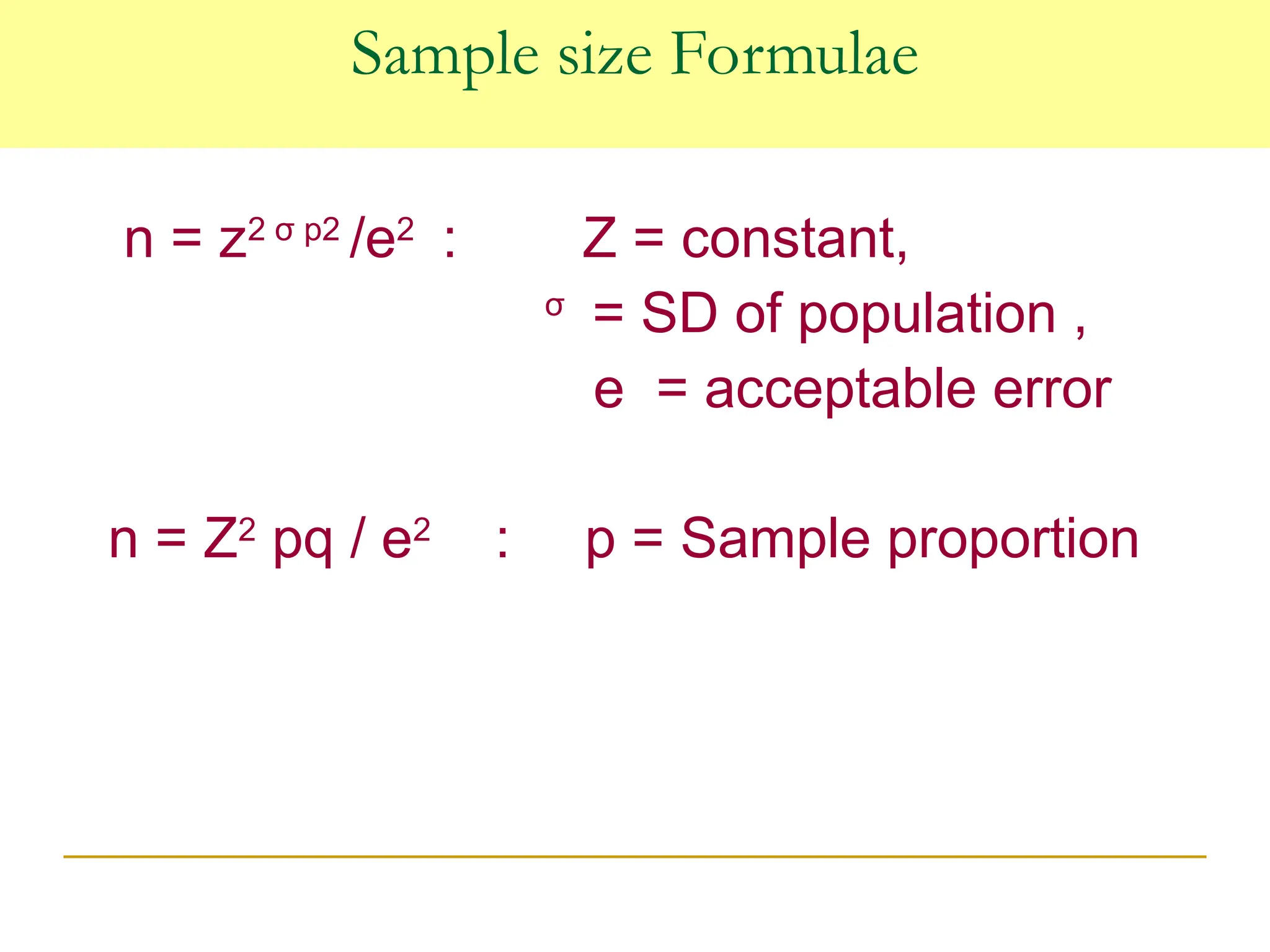
Sample size Formulae
n = z2 σ p2
/e2
: Z = constant,
σ
= SD of population ,
e = acceptable error
n = Z2
pq / e2
: p = Sample proportion

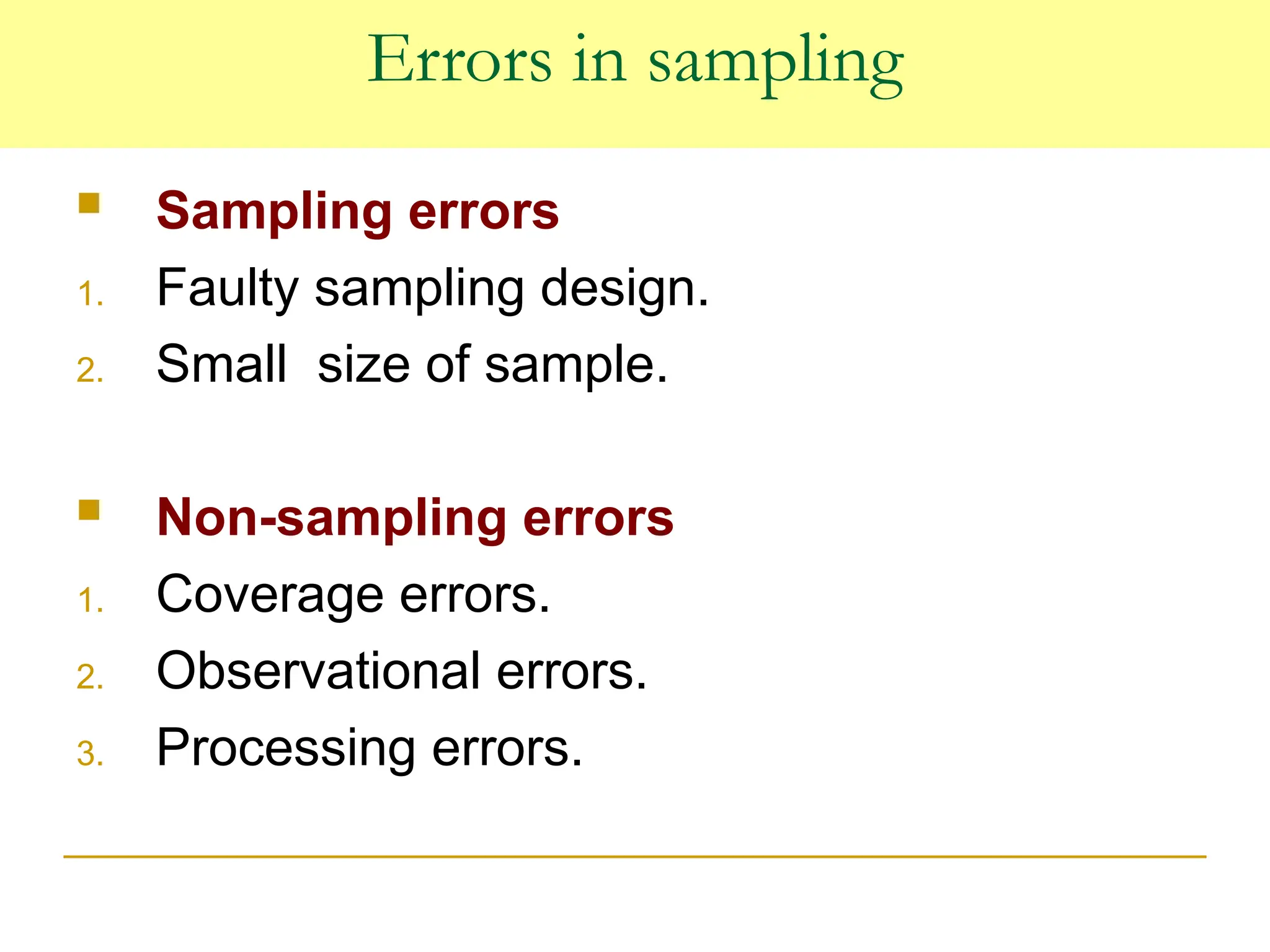
Errors in sampling
 Sampling errors
1. Faulty sampling design.
2. Small size of sample.
 Non-sampling errors
1. Coverage errors.
2. Observational errors.
3. Processing errors.

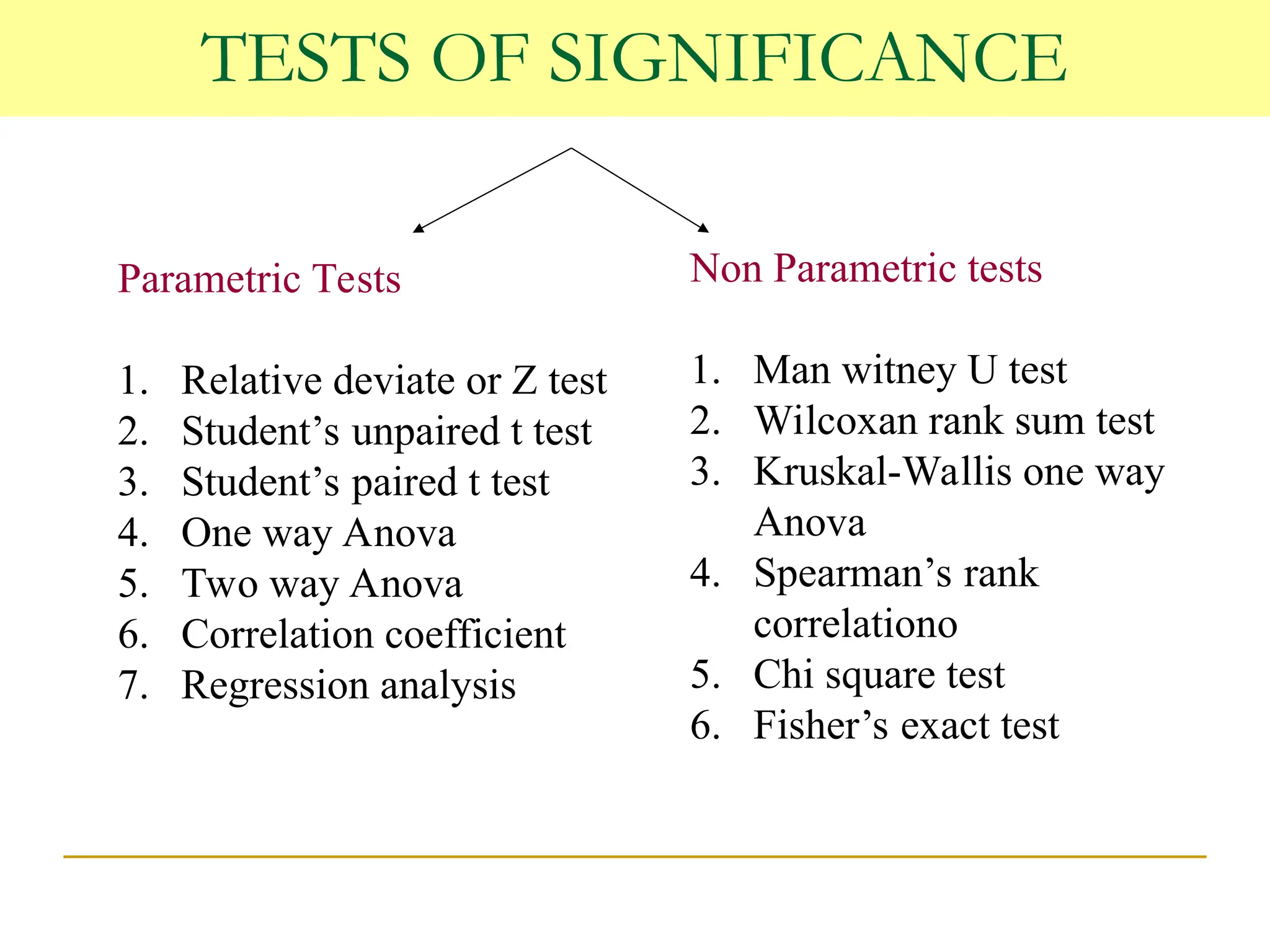
TESTS OF SIGNIFICANCE
Parametric Tests
1. Relative deviate or Z test
2. Student’s unpaired t test
3. Student’s paired t test
4. One way Anova
5. Two way Anova
6. Correlation coefficient
7. Regression analysis
Non Parametric tests
1. Man witney U test
2. Wilcoxan rank sum test
3. Kruskal-Wallis one way
Anova
4. Spearman’s rank
correlationo
5. Chi square test
6. Fisher’s exact test

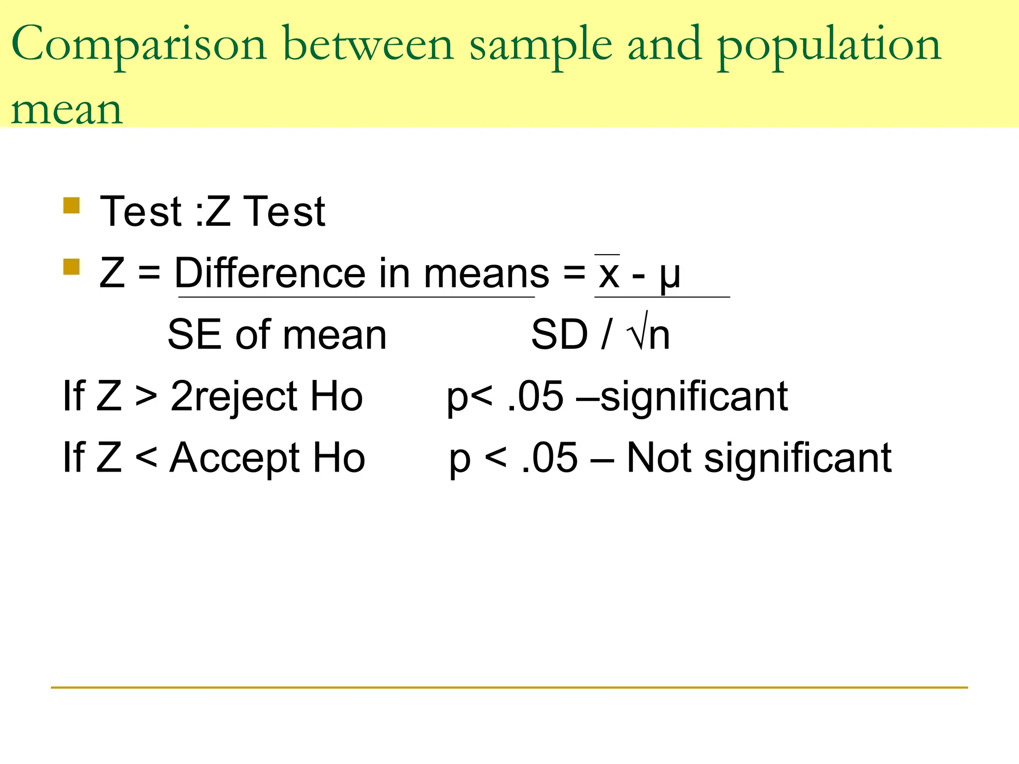
Comparison between sample and population
mean
 Test :Z Test
 Z = Difference in means = x - µ
SE of mean SD / √n
If Z > 2reject Ho p< .05 –significant
If Z < Accept Ho p < .05 – Not significant

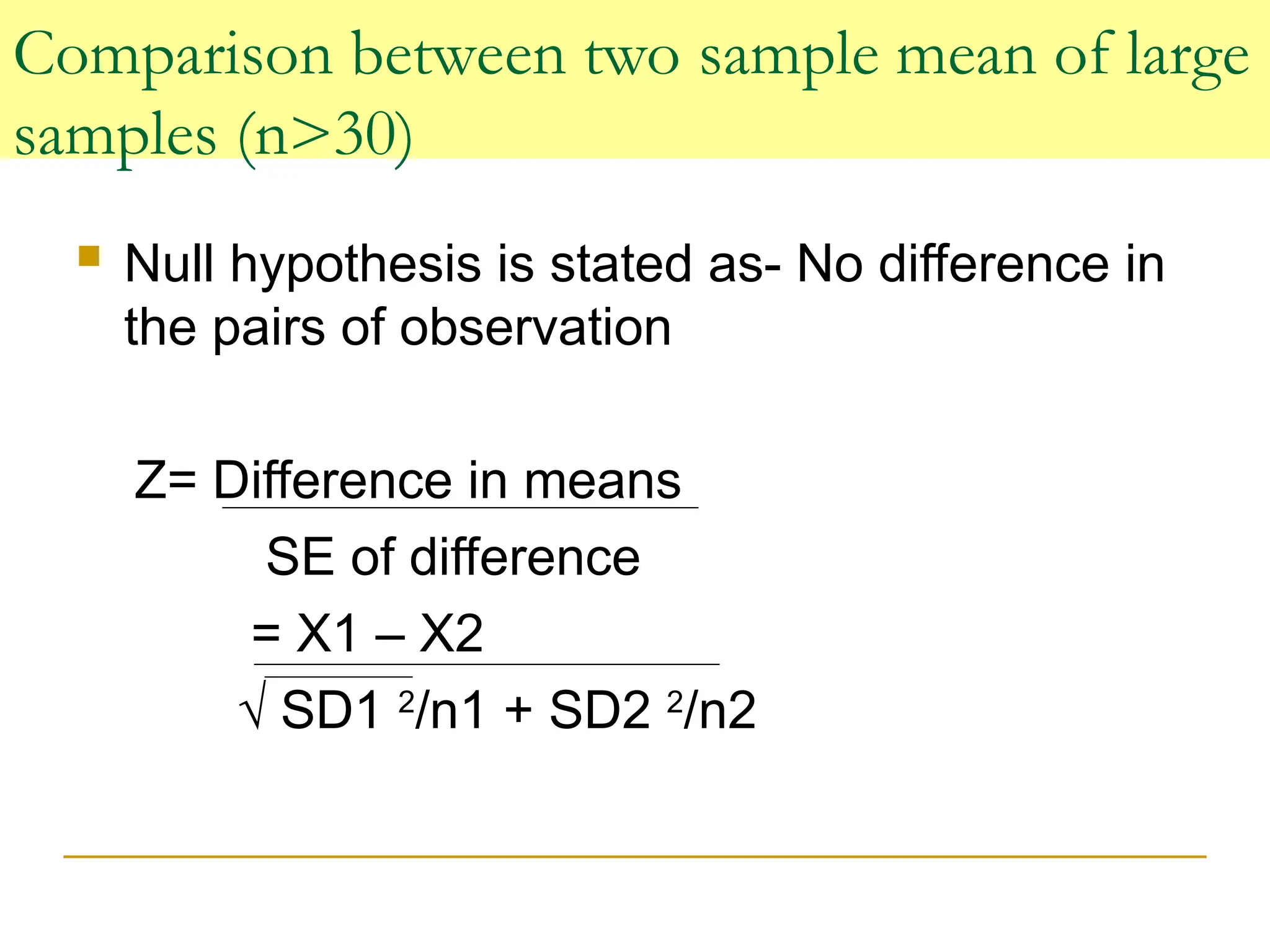
Comparison between two sample mean of large
samples (n>30)
 Null hypothesis is stated as- No difference in
the pairs of observation
Z= Difference in means
SE of difference
= X1 – X2
√ SD1 2
/n1 + SD2 2
/n2

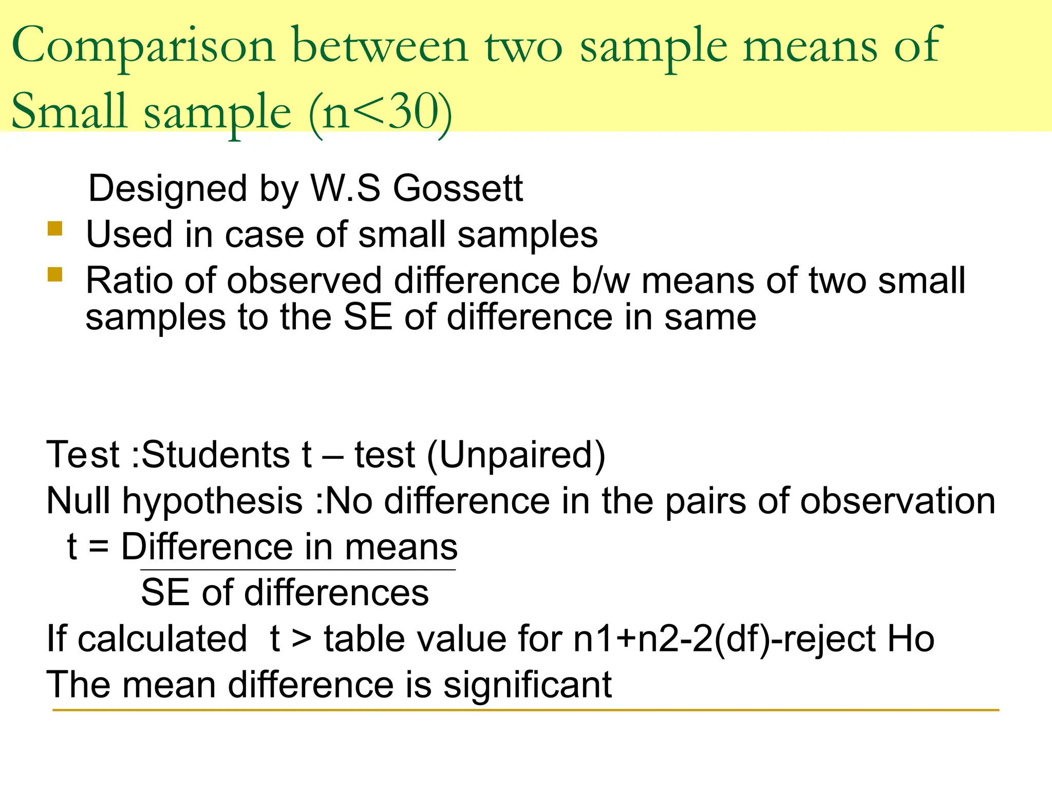
Comparison between two sample means of
Small sample (n<30)
Designed by W.S Gossett
 Used in case of small samples
 Ratio of observed difference b/w means of two small
samples to the SE of difference in same
Test :Students t – test (Unpaired)
Null hypothesis :No difference in the pairs of observation
t = Difference in means
SE of differences
If calculated t > table value for n1+n2-2(df)-reject Ho
The mean difference is significant

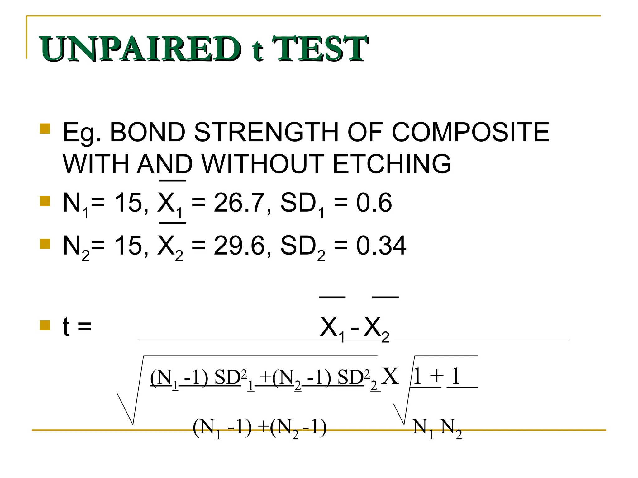
UNPAIRED t TEST
UNPAIRED t TEST
 Eg. BOND STRENGTH OF COMPOSITE
WITH AND WITHOUT ETCHING
 N1= 15, X1 = 26.7, SD1 = 0.6
 N2= 15, X2 = 29.6, SD2 = 0.34
 t = X1 - X2
(N1 -1) SD2
1 +(N2 -1) SD2
2 X 1 + 1
(N1 -1) +(N2 -1) N1 N2

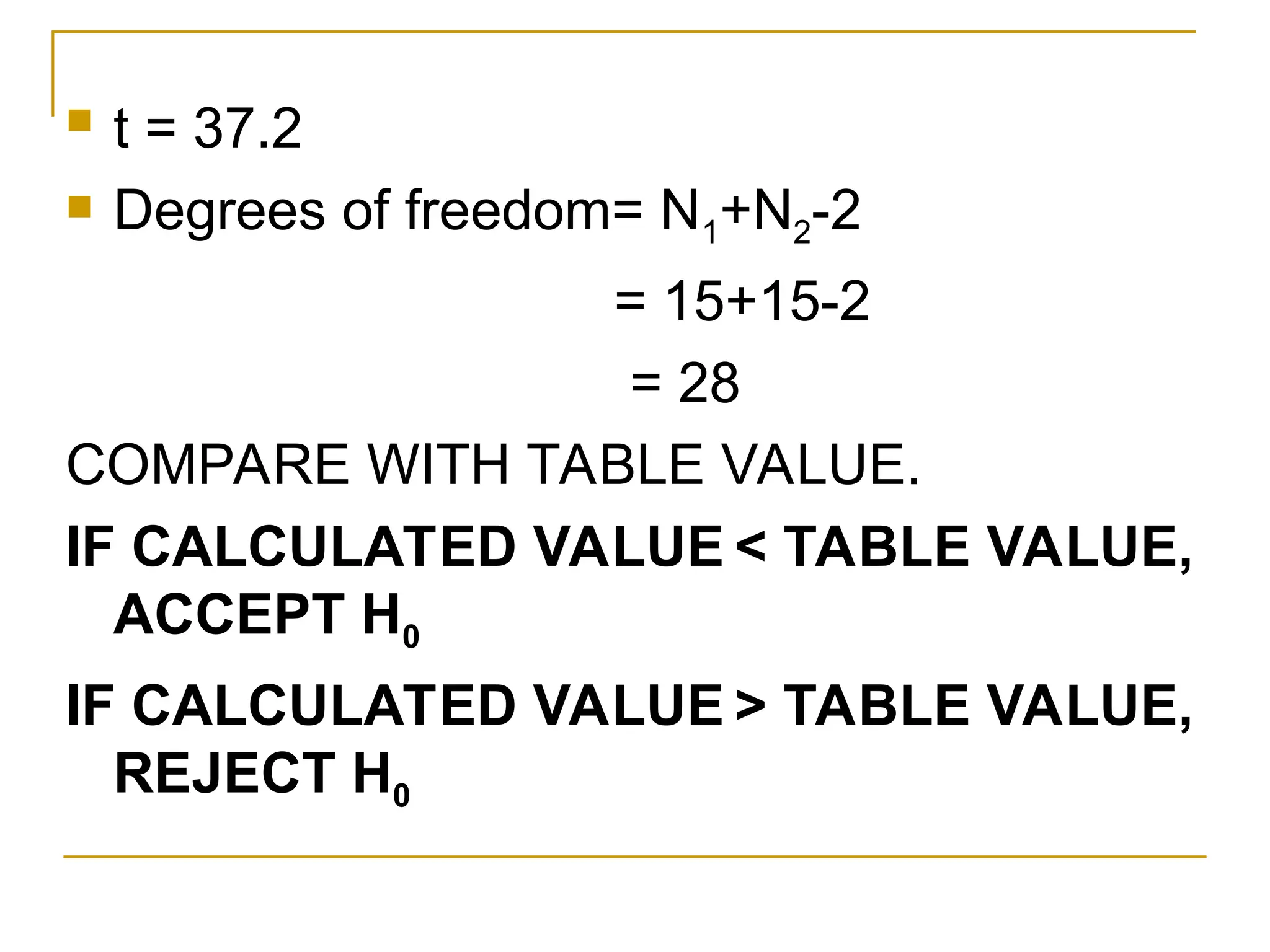
 t = 37.2
 Degrees of freedom= N1+N2-2
= 15+15-2
= 28
COMPARE WITH TABLE VALUE.
IF CALCULATED VALUE < TABLE VALUE,
ACCEPT H0
IF CALCULATED VALUE > TABLE VALUE,
REJECT H0

Student’s paired t test
 When each individual gives a pair of observations ,
and to test for difference in pair of values , paired ‘t’
test utilized
 t = Mean of differences /SE of difference

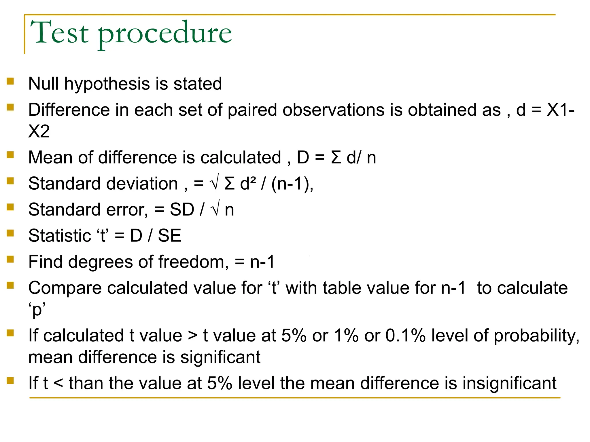
Test procedure
 Null hypothesis is stated
 Difference in each set of paired observations is obtained as , d = X1-
X2
 Mean of difference is calculated , D = Σ d/ n
 Standard deviation , = √ Σ d² / (n-1),
 Standard error, = SD / √ n
 Statistic ‘t’ = D / SE
 Find degrees of freedom, = n-1
 Compare calculated value for ‘t’ with table value for n-1 to calculate
‘p’
 If calculated t value > t value at 5% or 1% or 0.1% level of probability,
mean difference is significant
 If t < than the value at 5% level the mean difference is insignificant

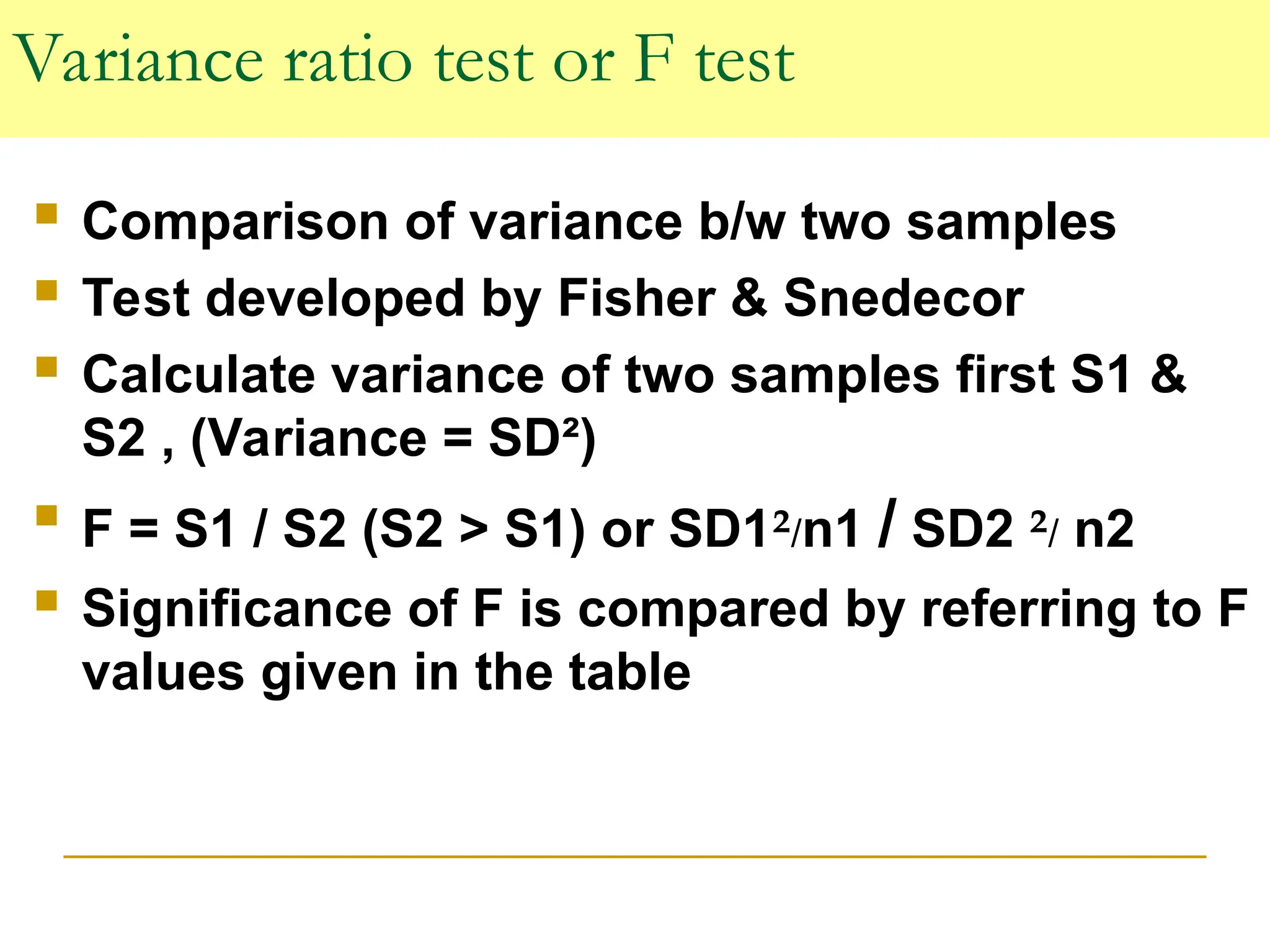
Variance ratio test or F test
 Comparison of variance b/w two samples
 Test developed by Fisher & Snedecor
 Calculate variance of two samples first S1 &
S2 , (Variance = SD²)

F = S1 / S2 (S2 > S1) or SD1²/n1 / SD2 ²/ n2
 Significance of F is compared by referring to F
values given in the table

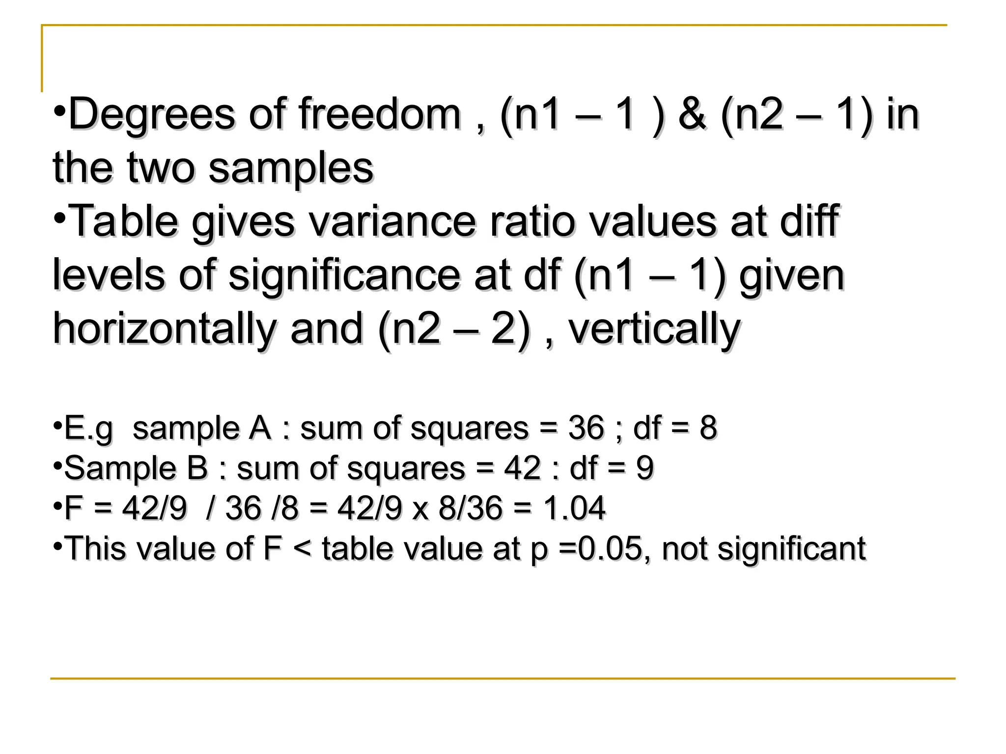
•Degrees of freedom , (n1 – 1 ) & (n2 – 1) in
Degrees of freedom , (n1 – 1 ) & (n2 – 1) in
the two samples
the two samples
•Table gives variance ratio values at diff
Table gives variance ratio values at diff
levels of significance at df (n1 – 1) given
levels of significance at df (n1 – 1) given
horizontally and (n2 – 2) , vertically
horizontally and (n2 – 2) , vertically
•E.g sample A : sum of squares = 36 ; df = 8
E.g sample A : sum of squares = 36 ; df = 8
•Sample B : sum of squares = 42 : df = 9
Sample B : sum of squares = 42 : df = 9
•F = 42/9 / 36 /8 = 42/9 x 8/36 = 1.04
F = 42/9 / 36 /8 = 42/9 x 8/36 = 1.04
•This value of F < table value at p =0.05, not significant
This value of F < table value at p =0.05, not significant

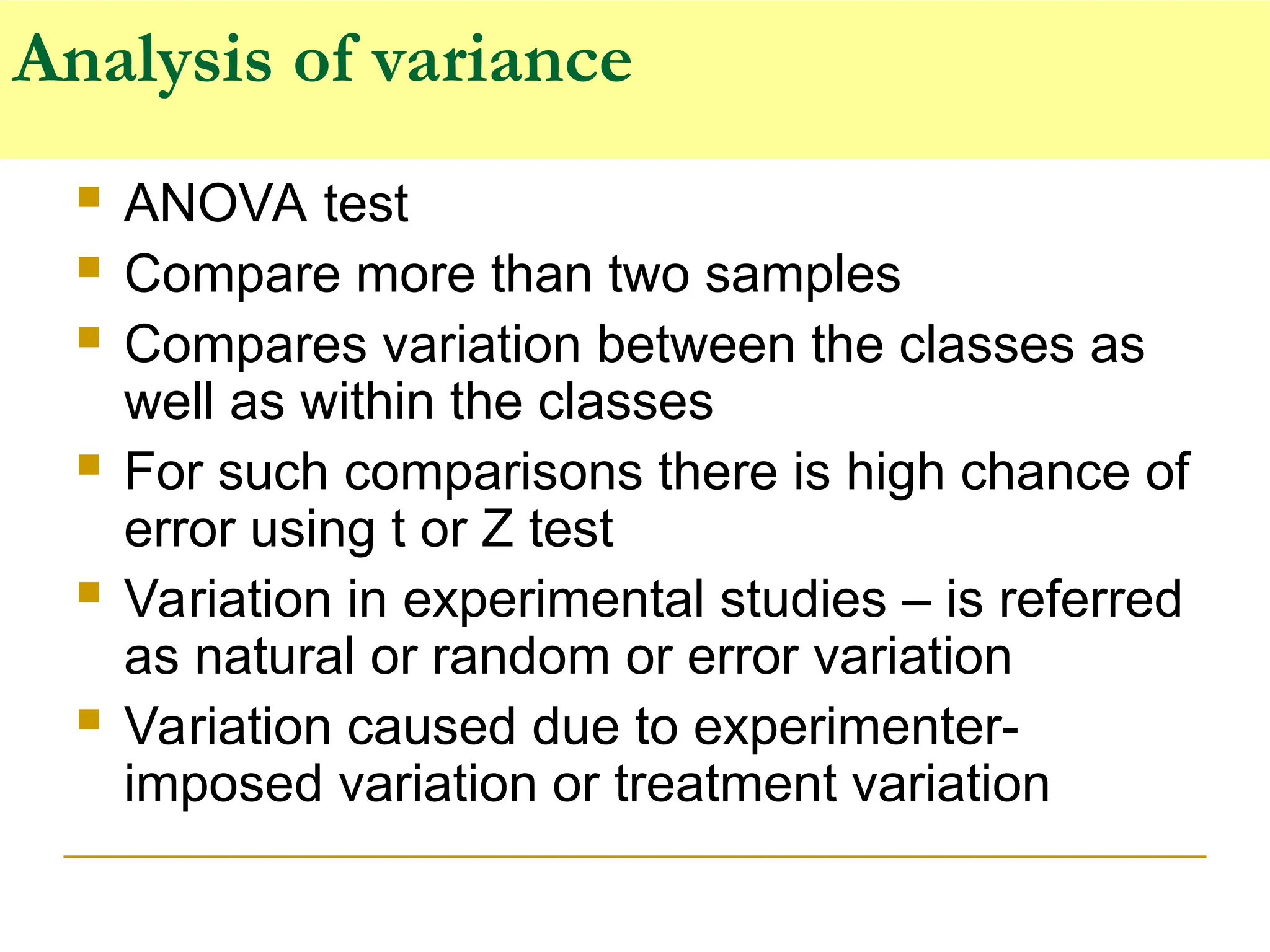
Analysis of variance
 ANOVA test
 Compare more than two samples
 Compares variation between the classes as
well as within the classes
 For such comparisons there is high chance of
error using t or Z test
 Variation in experimental studies – is referred
as natural or random or error variation
 Variation caused due to experimenter-
imposed variation or treatment variation

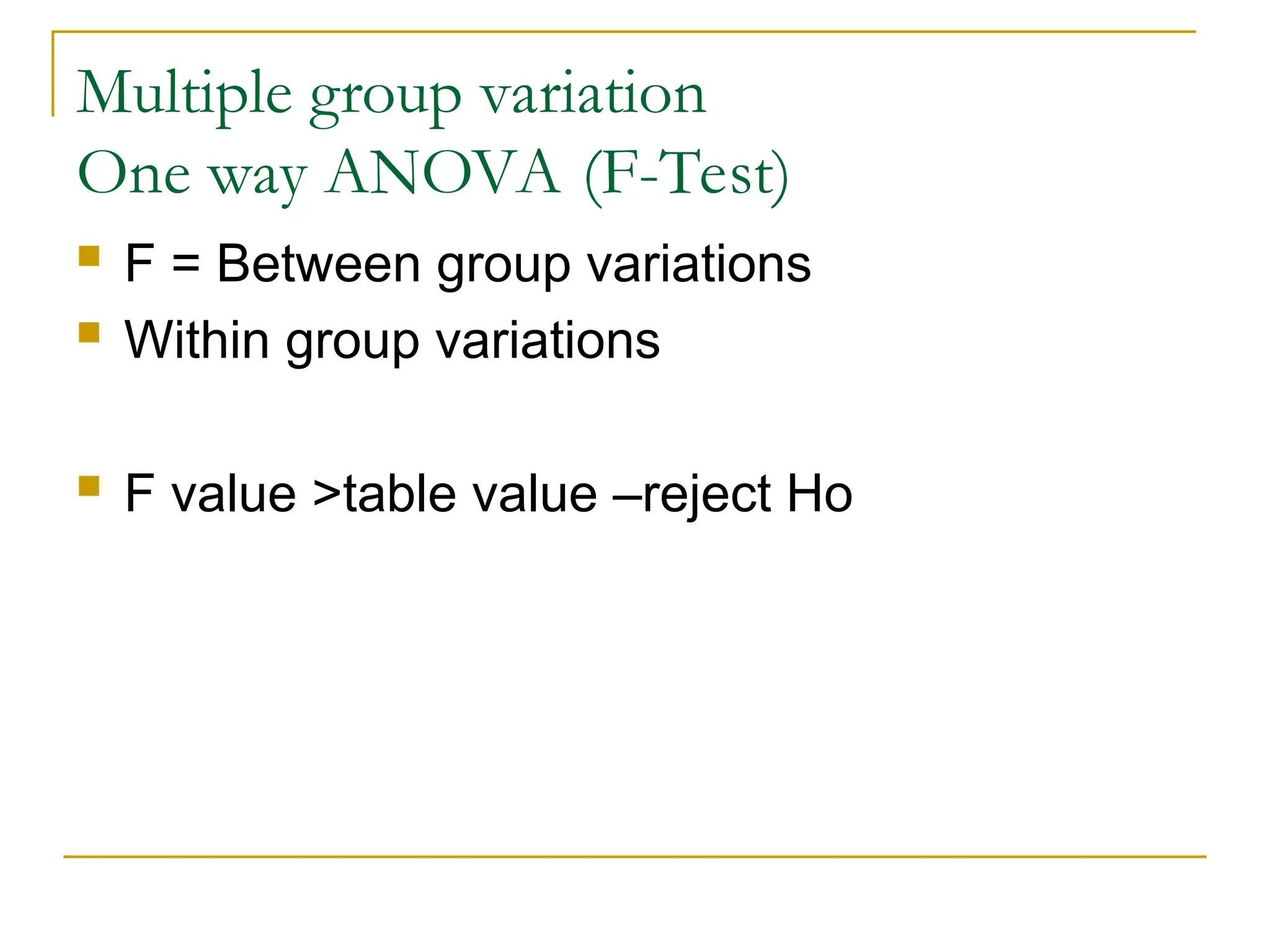
Multiple group variation
One way ANOVA (F-Test)
 F = Between group variations
 Within group variations
 F value >table value –reject Ho

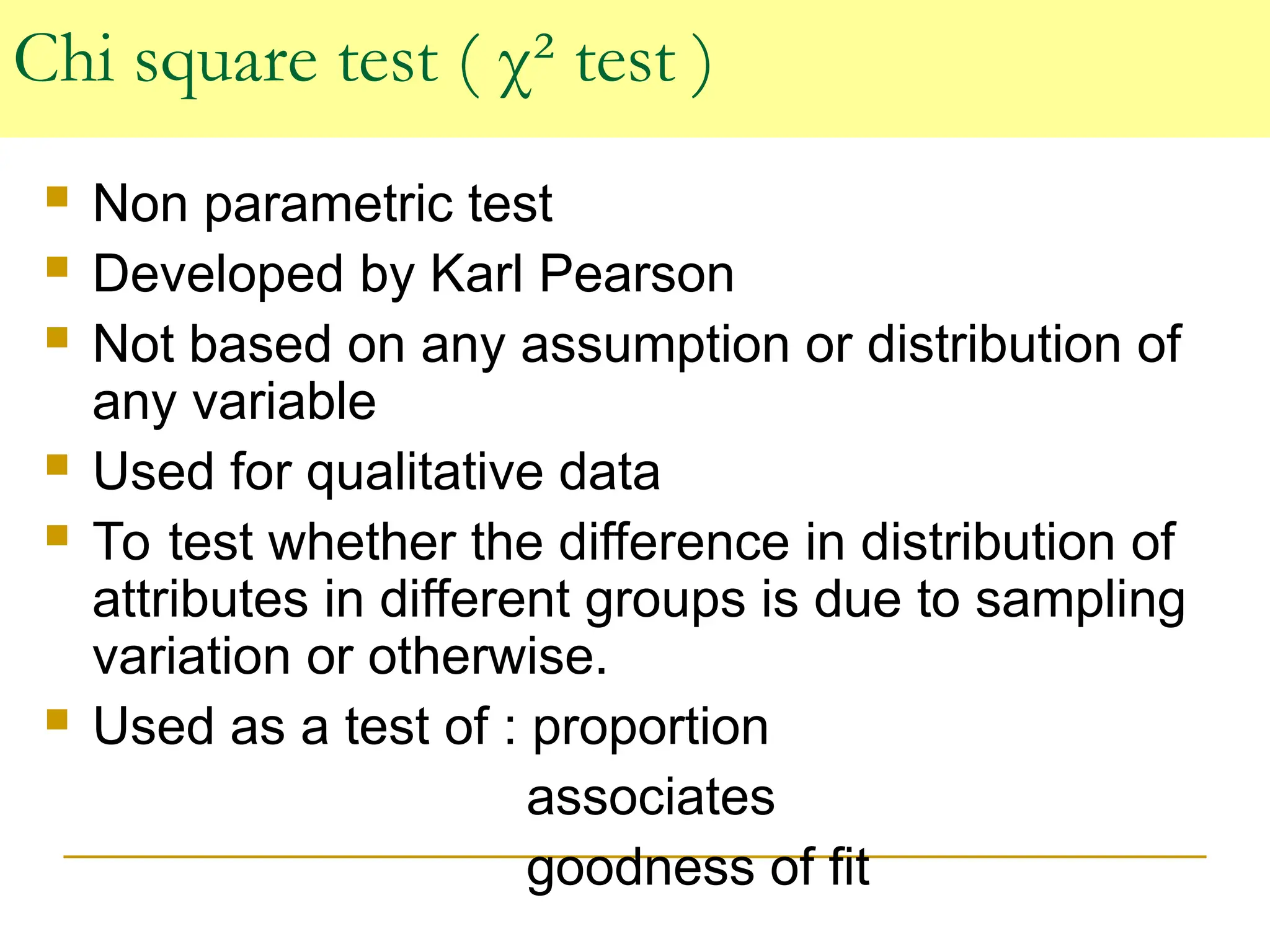
Chi square test ( χ² test )
 Non parametric test
 Developed by Karl Pearson
 Not based on any assumption or distribution of
any variable
 Used for qualitative data
 To test whether the difference in distribution of
attributes in different groups is due to sampling
variation or otherwise.
 Used as a test of : proportion
associates
goodness of fit

Test of proportions
 Find the significance of difference in two or more than two
proportions.
 To compare values of two binomial samples even when
they are very small (< 30)
 To compare the frequencies of two multinomial samples
Test of association
 Association b/w two events in binomial or multinomial
samples
 Measures the probability of association b/w two discrete
variables
 Assumption of independence made unless proved
otherwise by χ² test

Test of goodness of fit
 It is to determine if the actual numbers are
similar to the expected or theoretical numbers
 Check whether the observed frequency
distribution fits in a hypothetical or theoretical
or assumed distribution
 Test the difference b/w observed & assumed
is by chance or due to a particular factor
 Also determines if the difference is by chance

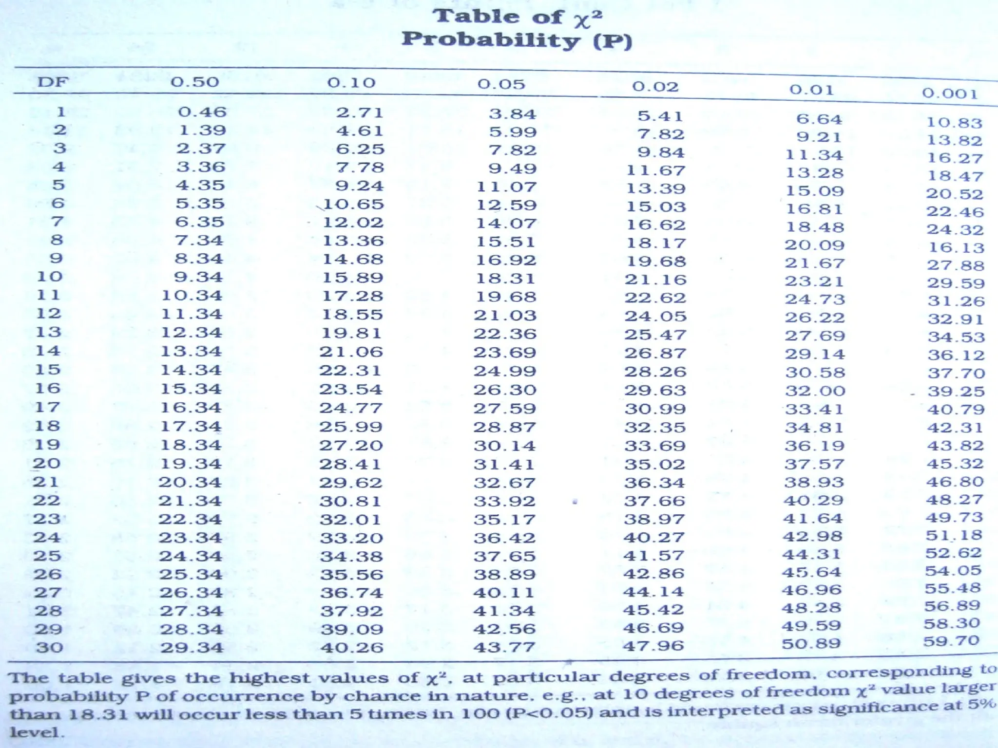
 If calculated chi square value > expected
value in table (at p = 0.05):-
 Hypothesis of no difference or hypothesis of
independence of two characters is rejected
 If calculated value lower – hypothesis not
rejected, concluding that difference is due to
chance or the two characters are not
associated
 Level of significance of χ² stated in
percentages as 5% , 1% ..

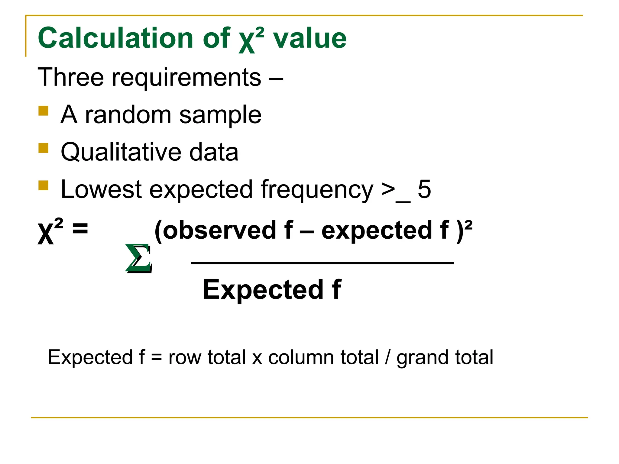
Calculation of χ² value
Three requirements –
 A random sample
 Qualitative data
 Lowest expected frequency >_ 5
χ² = (observed f – expected f )²
Σ
Σ
Expected f
Expected f = row total x column total / grand total

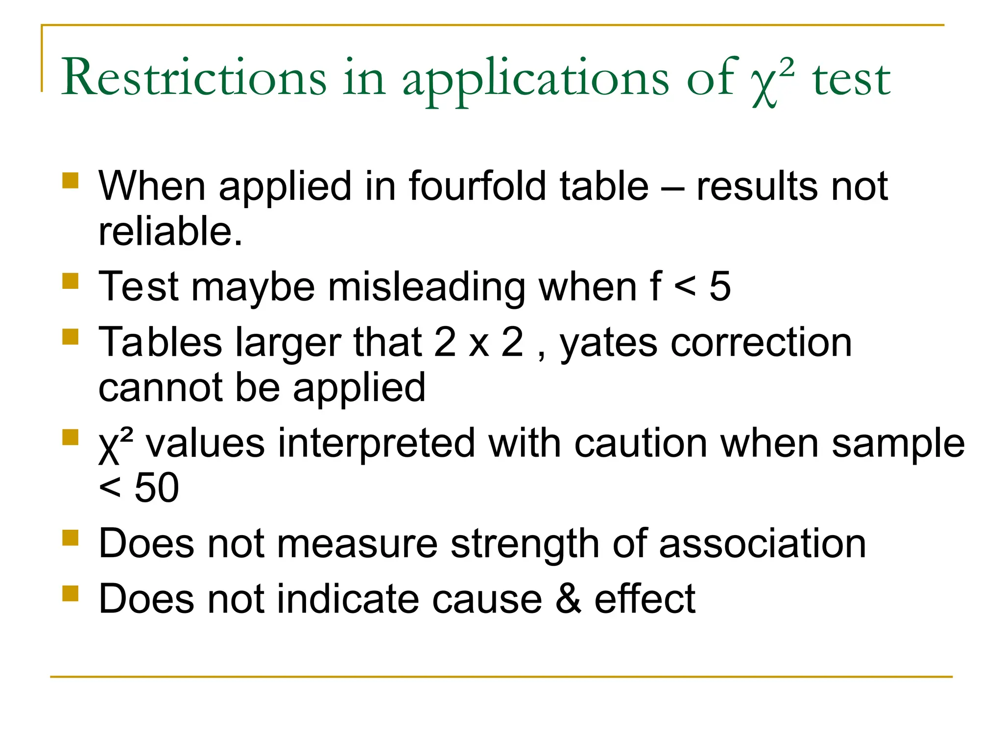
Restrictions in applications of χ² test
 When applied in fourfold table – results not
reliable.
 Test maybe misleading when f < 5
 Tables larger that 2 x 2 , yates correction
cannot be applied
 χ² values interpreted with caution when sample
< 50
 Does not measure strength of association
 Does not indicate cause & effect

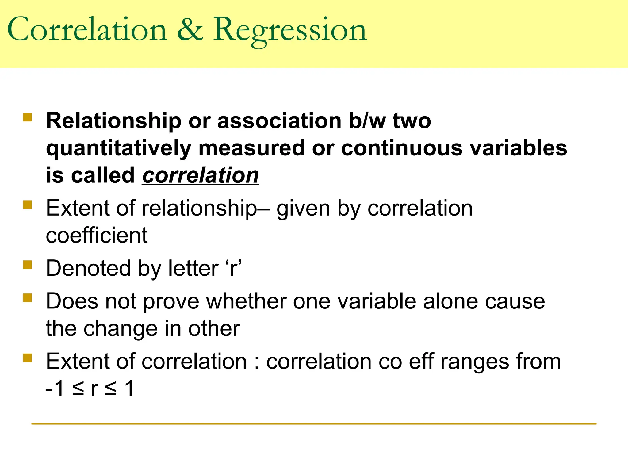
Correlation & Regression
 Relationship or association b/w two
quantitatively measured or continuous variables
is called correlation
 Extent of relationship– given by correlation
coefficient
 Denoted by letter ‘r’
 Does not prove whether one variable alone cause
the change in other
 Extent of correlation : correlation co eff ranges from
-1 ≤ r ≤ 1

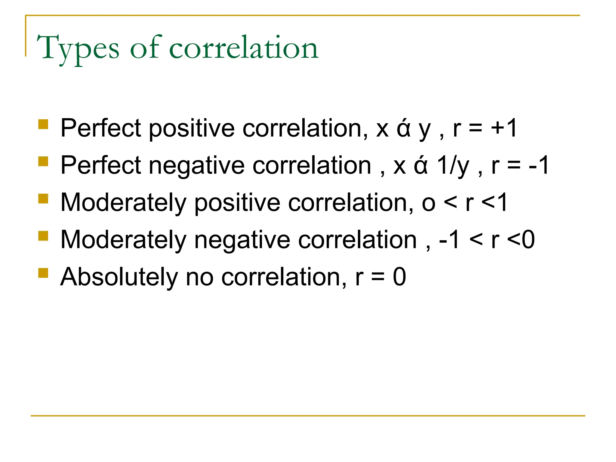
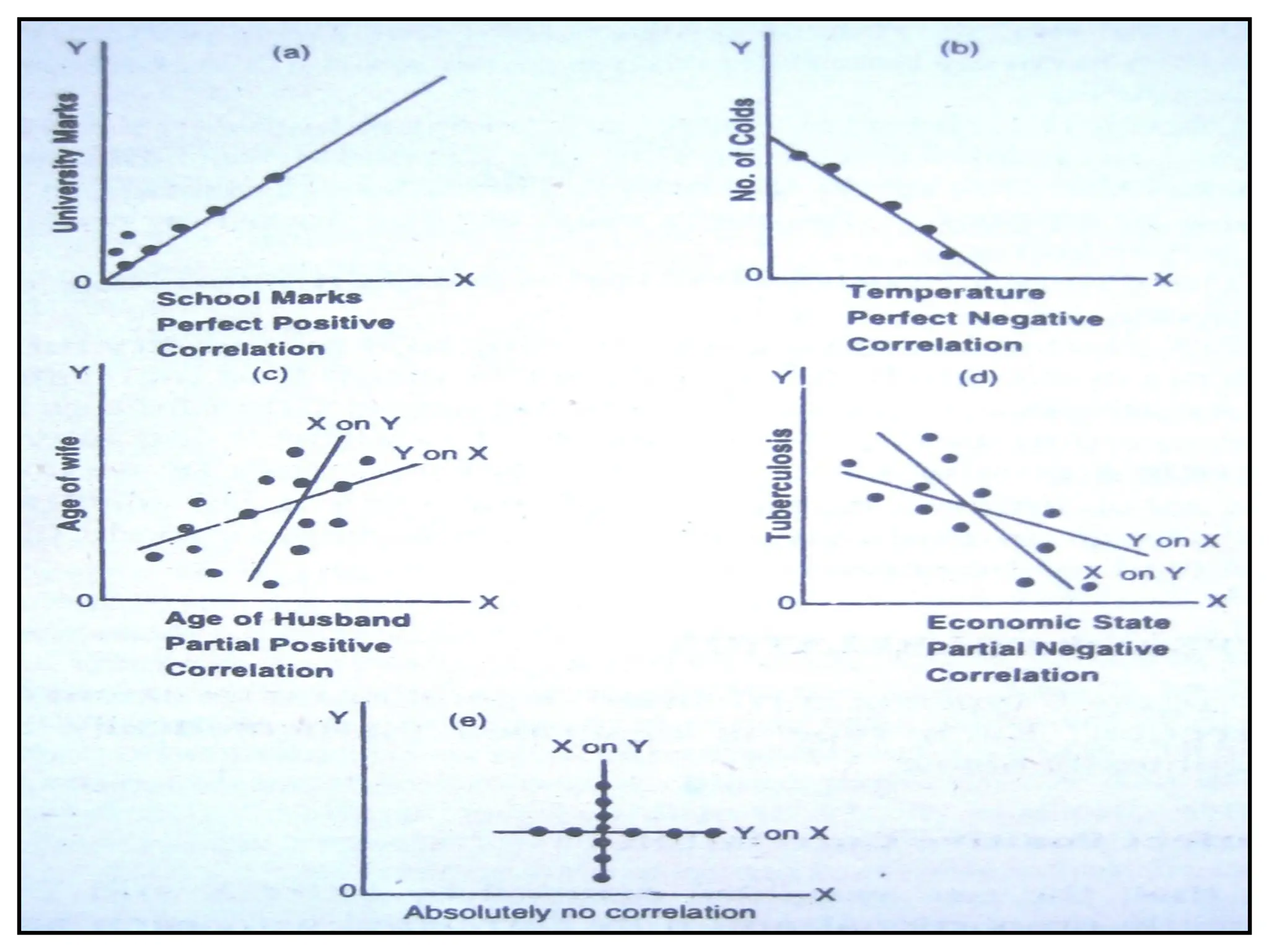
Types of correlation
 Perfect positive correlation, x ά y , r = +1
 Perfect negative correlation , x ά 1/y , r = -1
 Moderately positive correlation, o < r <1
 Moderately negative correlation , -1 < r <0
 Absolutely no correlation, r = 0

Calculation of correlation coefficient
 Pearson’s correlation coefficient
 r = Σ (X – x) (Y-y)
√ Σ (X –x)² Σ (Y- y)²

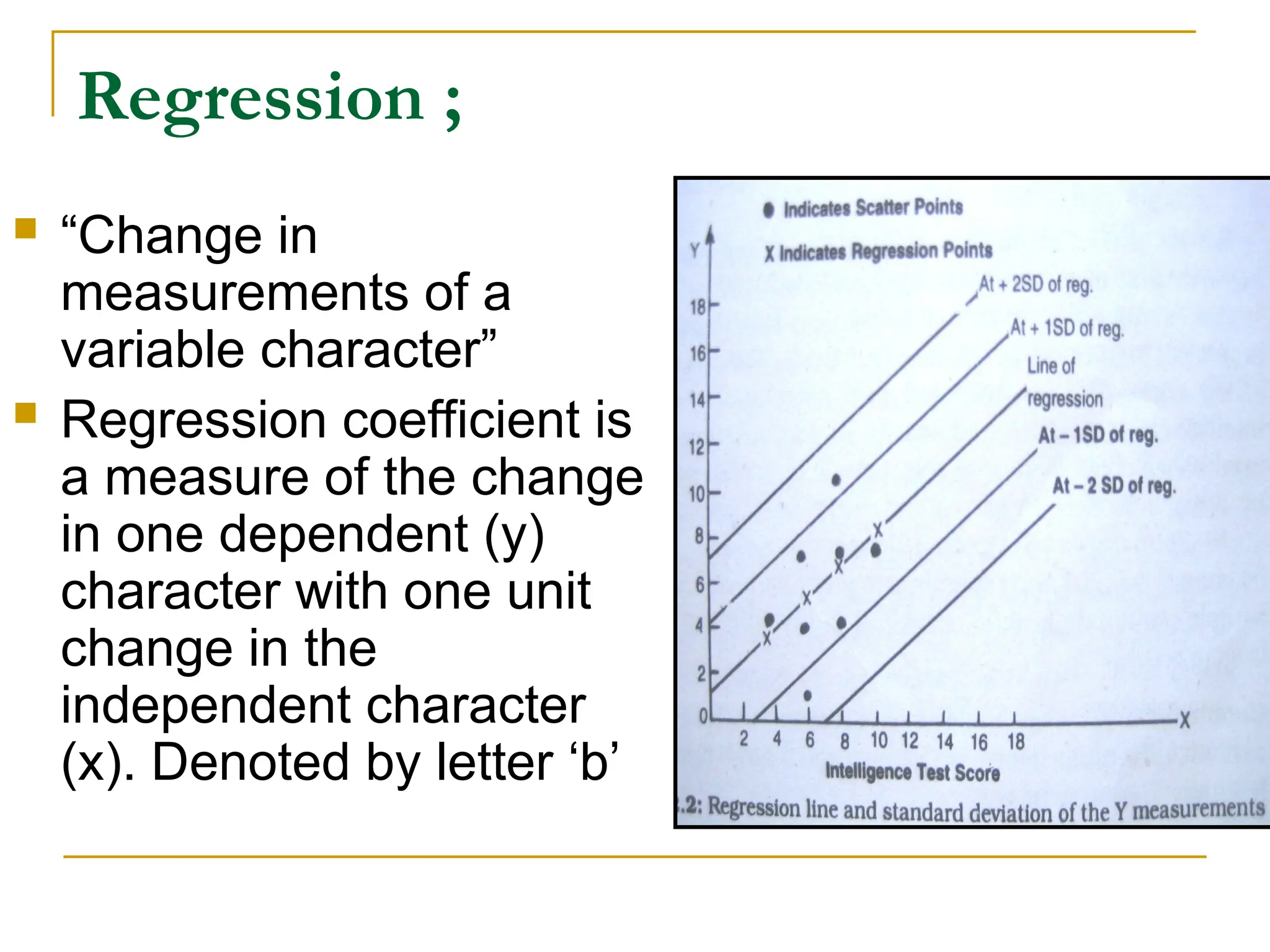
Regression ;
 “Change in
measurements of a
variable character”
 Regression coefficient is
a measure of the change
in one dependent (y)
character with one unit
change in the
independent character
(x). Denoted by letter ‘b’

Non parametric tests
 Friedman’s test – nonparametric equivalent of analysis of
variance
 Kruskal – Wallis test – to compare medians of several
independent samples equivalent of one –way analysis of
variance
 Mann – Whitney U test – compare medians of two
independent samples. Equivalent of t test
 McNemar’s test variant of chi squared test , used when data
is paired
 Sign test – paired data
 Spearman’s rank correlation – correlation coefficient
A family of statistical tests also called as distribution free tests
A family of statistical tests also called as distribution free tests
that do not require any assumption about the distribution the
that do not require any assumption about the distribution the
data set follows and that do not require the testing of
data set follows and that do not require the testing of
distribution parameters such as means or variances
distribution parameters such as means or variances

REFERENCES;
1. Text book of biostatistics- Bhaskara Rao
2. Text book of biostatistics- Indryan
3. Text book of biostatistics- Prabhakar
4. Essential of preventive and community
dentistry- Soben Peter
5. Park and park

intro to biostatistics and data variables (2).ppt

intro to biostatistics and data variables (2).ppt

More Related Content

Similar to intro to biostatistics and data variables (2).ppt

Recently uploaded

intro to biostatistics and data variables (2).ppt

Editor's Notes