![Today’s Agenda
(IF, Nested IF, VLOOKUP, HLOOKUP)
- Formulas and Functions
- List of Formulas [Practical]
- 15 Important Functions for Data Analysis+ Practice
- Error Handling
- Data Validation
- Macro
09-Sep-20
Content sources are mentioned in bottom 03 Slides |
redwan.contact@gmail.com
2](https://image.slidesharecdn.com/basicdataanalysisforsmeusingmsexcelday-03-200910045123/75/Elementary-Data-Analysis-with-MS-Excel_Day-3-2-2048.jpg)
![DAYS/NETWORKDAYS
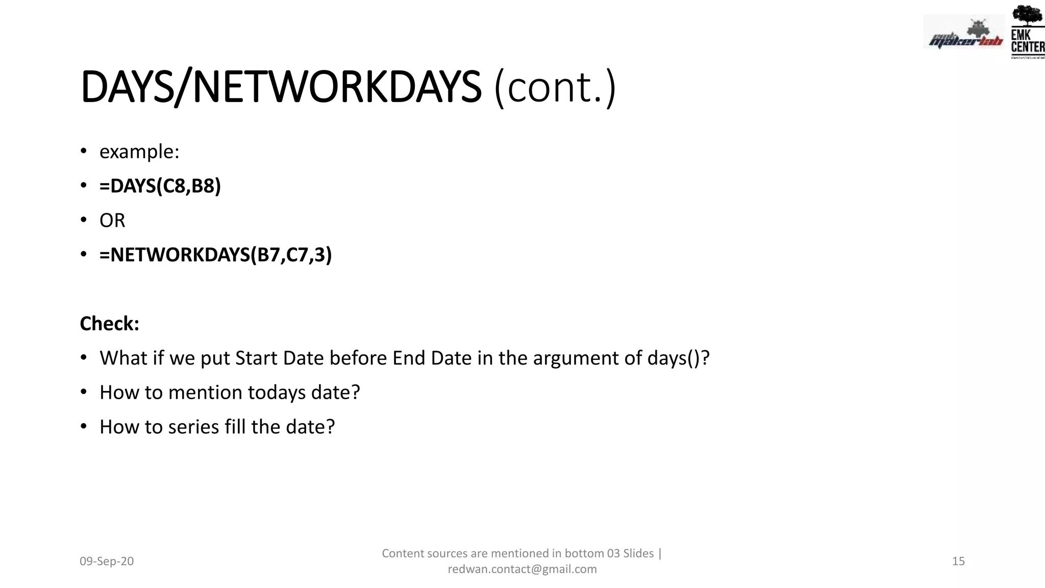
• =DAYS is exactly what it implies. This function determines the number of calendar days between
two dates. This is a useful tool for assessing the lifecycle of products, contracts, and run rating
revenue depending on service length – a data analysis essential.
=NETWORKDAYS is slightly more robust and useful. This formula determines the number of
“workdays” between two dates as well as an option to account for holidays. Even workaholics
need a break now and then! Using these two formulas to compare time frames is especially
helpful for project management.
• Formulas:
=DAYS(SELECT CELL, SELECT CELL)
• OR
=NETWORKDAYS(SELECT CELL, SELECT CELL,[numberofholidays])
note: [numberofholidays] is optional
09-Sep-20
Content sources are mentioned in bottom 03 Slides |
redwan.contact@gmail.com
14](https://image.slidesharecdn.com/basicdataanalysisforsmeusingmsexcelday-03-200910045123/75/Elementary-Data-Analysis-with-MS-Excel_Day-3-14-2048.jpg)
![SUMIFS
• =SUMIFS is one of the “must-know” formulas for a data analyst. The
common formula used is =SUM, but what if you need to sum values based
on multiple criteria? SUMIFS is it. In the example below, SUMIFS is used to
determine how much each product is contributing to top-line revenue.
• Formula:
=SUMIFS (sum_range, range1, criteria1, [range2], [criteria2], ...)
• example:
= SUMIFS(F5:F11,C5:C11,"red") // sum if red
= SUMIFS(F5:F11,C5:C11,"red",D5:D11,"TX") // sum if red and TX
09-Sep-20
Content sources are mentioned in bottom 03 Slides |
redwan.contact@gmail.com
16](https://image.slidesharecdn.com/basicdataanalysisforsmeusingmsexcelday-03-200910045123/75/Elementary-Data-Analysis-with-MS-Excel_Day-3-16-2048.jpg)
![SUMIFS (cont.)
Arguments:
• sum_range - The range to be summed.
• range1 - The first range to evaluate.
• criteria1 - The criteria to use on range1.
• range2 - [optional] The second range to evaluate.
• criteria2 - [optional] The criteria to use on range2.
09-Sep-20
Content sources are mentioned in bottom 03 Slides |
redwan.contact@gmail.com
17](https://image.slidesharecdn.com/basicdataanalysisforsmeusingmsexcelday-03-200910045123/75/Elementary-Data-Analysis-with-MS-Excel_Day-3-17-2048.jpg)
![AVERAGEIFS
• Much like SUMIFS, AVERAGEIFS allows you to take an average based
on one or more criteria.
Formula:
• =AVERAGEIF(SELECT CELL, CRITERIA,[AVERAGE_RANGE])
• note: [average_range] is optional
• example:
• =AVERAGEIF($C:$C,$A:$A,$F2)
09-Sep-20
Content sources are mentioned in bottom 03 Slides |
redwan.contact@gmail.com
19](https://image.slidesharecdn.com/basicdataanalysisforsmeusingmsexcelday-03-200910045123/75/Elementary-Data-Analysis-with-MS-Excel_Day-3-19-2048.jpg)
![VLOOKUP
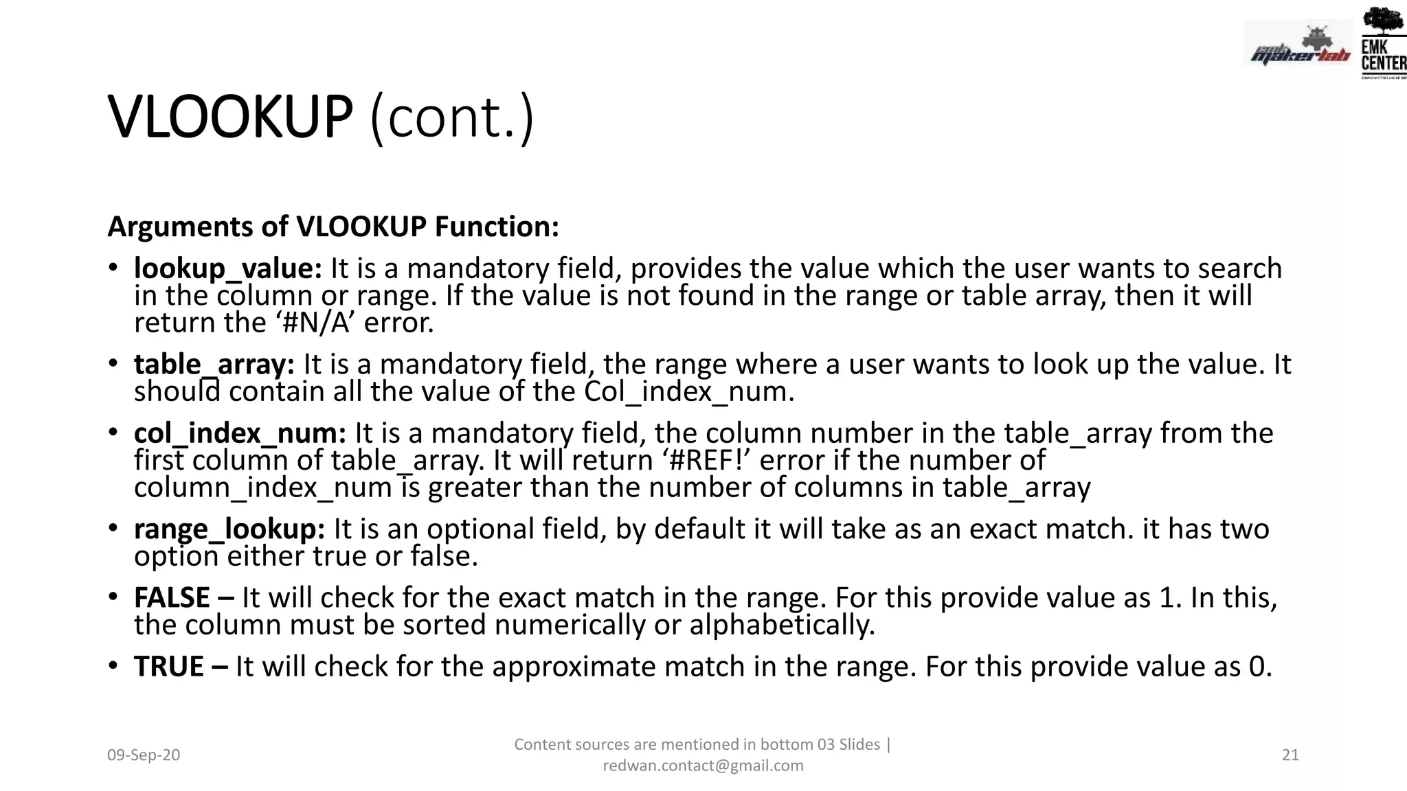
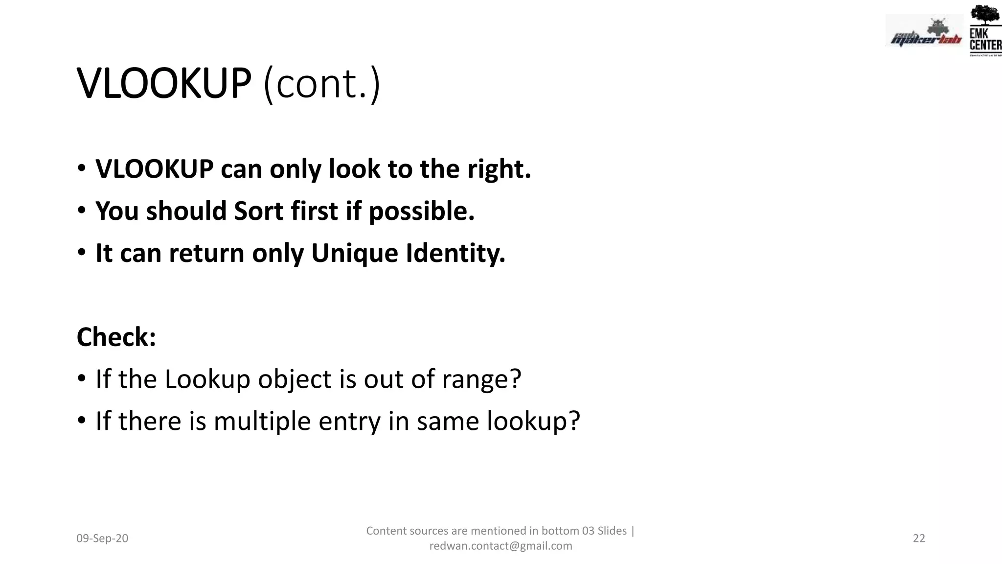
• VLOOKUP is one of the most useful and recognizable data analysis
functions. As an Excel user, you’ll probably need to “marry” data together
at some point. For example, accounts receivable might know how much
each product costs, but the shipping department can only provide units
shipped. This is the perfect use case for VLOOKUP.
Formula:
• =VLOOKUP(LOOKUP_VALUE,TABLE_ARRAY,COL_INDEX_NUM,
[RANGE_LOOKUP])
• example:
• =VLOOKUP(A5,$A$1:$G$44,3)
09-Sep-20
Content sources are mentioned in bottom 03 Slides |
redwan.contact@gmail.com
20](https://image.slidesharecdn.com/basicdataanalysisforsmeusingmsexcelday-03-200910045123/75/Elementary-Data-Analysis-with-MS-Excel_Day-3-20-2048.jpg)
![FIND/SEARCH
• =FIND/=SEARCH are powerful functions for isolating specific text within a data
set. Both are listed here because =FIND will return a case-sensitive match, i.e. if
you use FIND to query for “Big” you will only return Big=true results. But a
=SEARCH for “Big” will match with Big or big, making the query a bit broader. This
is particularly useful for looking for anomalies or unique identifiers.
Formula:
• =FIND(TEXT,WITHIN_TEXT,[START_NUMBER]) OR
=SEARCH(TEXT,WITHIN_TEXT,[START_NUMBER])
• note: [start_number] is optional and is used to indicate the starting cell in the text
to search
• example:
• =(FIND(“Central”, B2))
09-Sep-20
Content sources are mentioned in bottom 03 Slides |
redwan.contact@gmail.com
24](https://image.slidesharecdn.com/basicdataanalysisforsmeusingmsexcelday-03-200910045123/75/Elementary-Data-Analysis-with-MS-Excel_Day-3-24-2048.jpg)
![RANK
• =RANK is an ancient excel function, but that doesn’t downplay its
effectiveness for data analysis. =RANK allows you to quickly denote how
values rank in a dataset in ascending or descending order. In the example,
RANK is being used to determine which clients order the most product.
Formula:
• =RANK(SELECT CELL,RANGE_TO_RANK_AGAINST,[ORDER])
• note: [order] is optional
• example:
• =RANK(H1,$H$1:$H$43)
09-Sep-20
Content sources are mentioned in bottom 03 Slides |
redwan.contact@gmail.com
32](https://image.slidesharecdn.com/basicdataanalysisforsmeusingmsexcelday-03-200910045123/75/Elementary-Data-Analysis-with-MS-Excel_Day-3-32-2048.jpg)

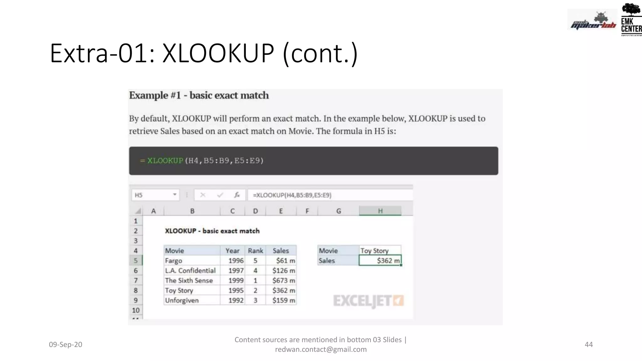
![Extra-01: XLOOKUP (Office365)
• The Excel XLOOKUP function is a modern and flexible replacement for
older functions like VLOOKUP, HLOOKUP, and LOOKUP. XLOOKUP
supports approximate and exact matching, wildcards (* ?) for partial
matches, and lookups in vertical or horizontal ranges.
• Syntax
=XLOOKUP (lookup, lookup_array, return_array, [not_found],
[match_mode], [search_mode])
09-Sep-20
Content sources are mentioned in bottom 03 Slides |
redwan.contact@gmail.com
40](https://image.slidesharecdn.com/basicdataanalysisforsmeusingmsexcelday-03-200910045123/75/Elementary-Data-Analysis-with-MS-Excel_Day-3-40-2048.jpg)
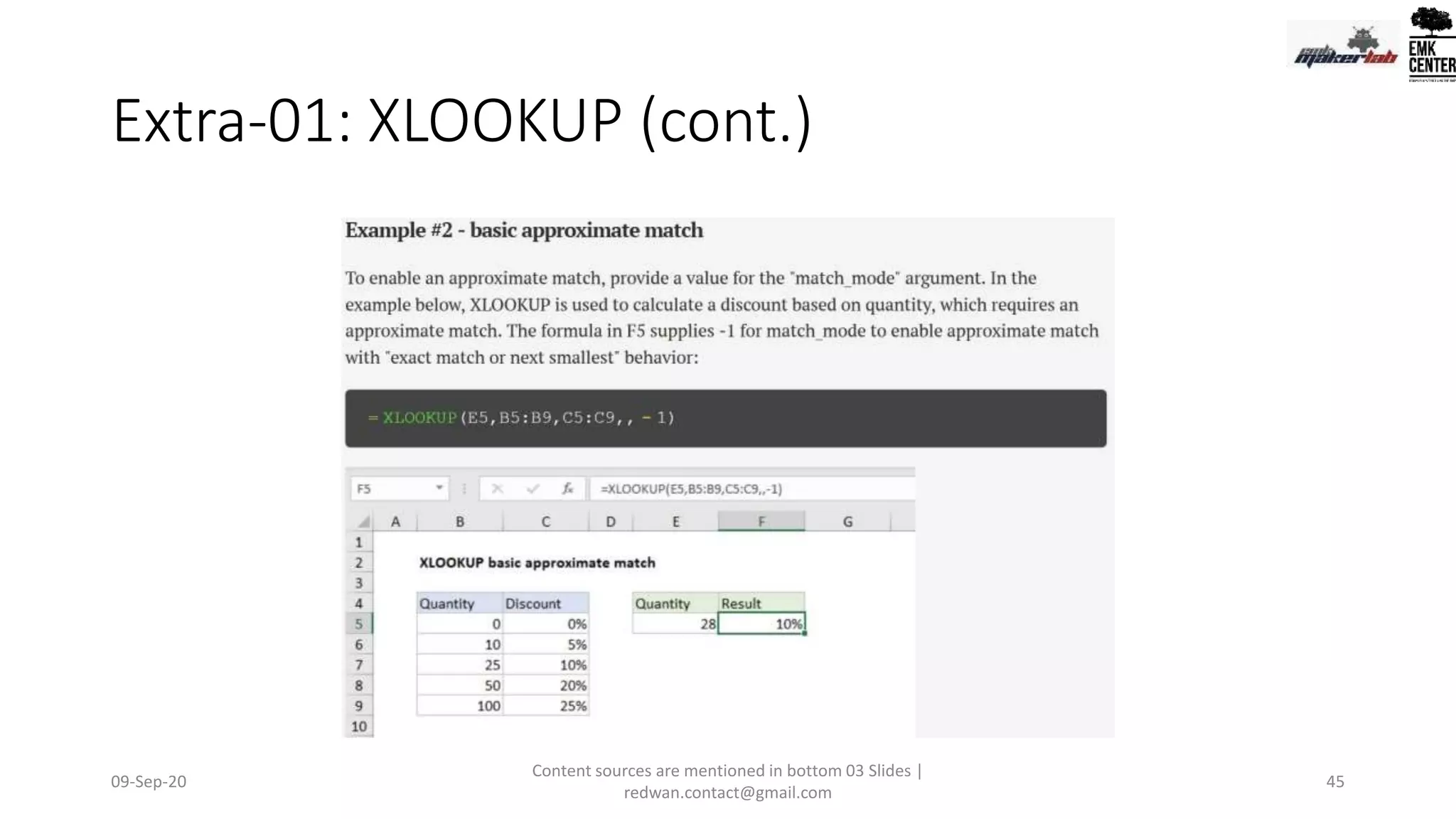
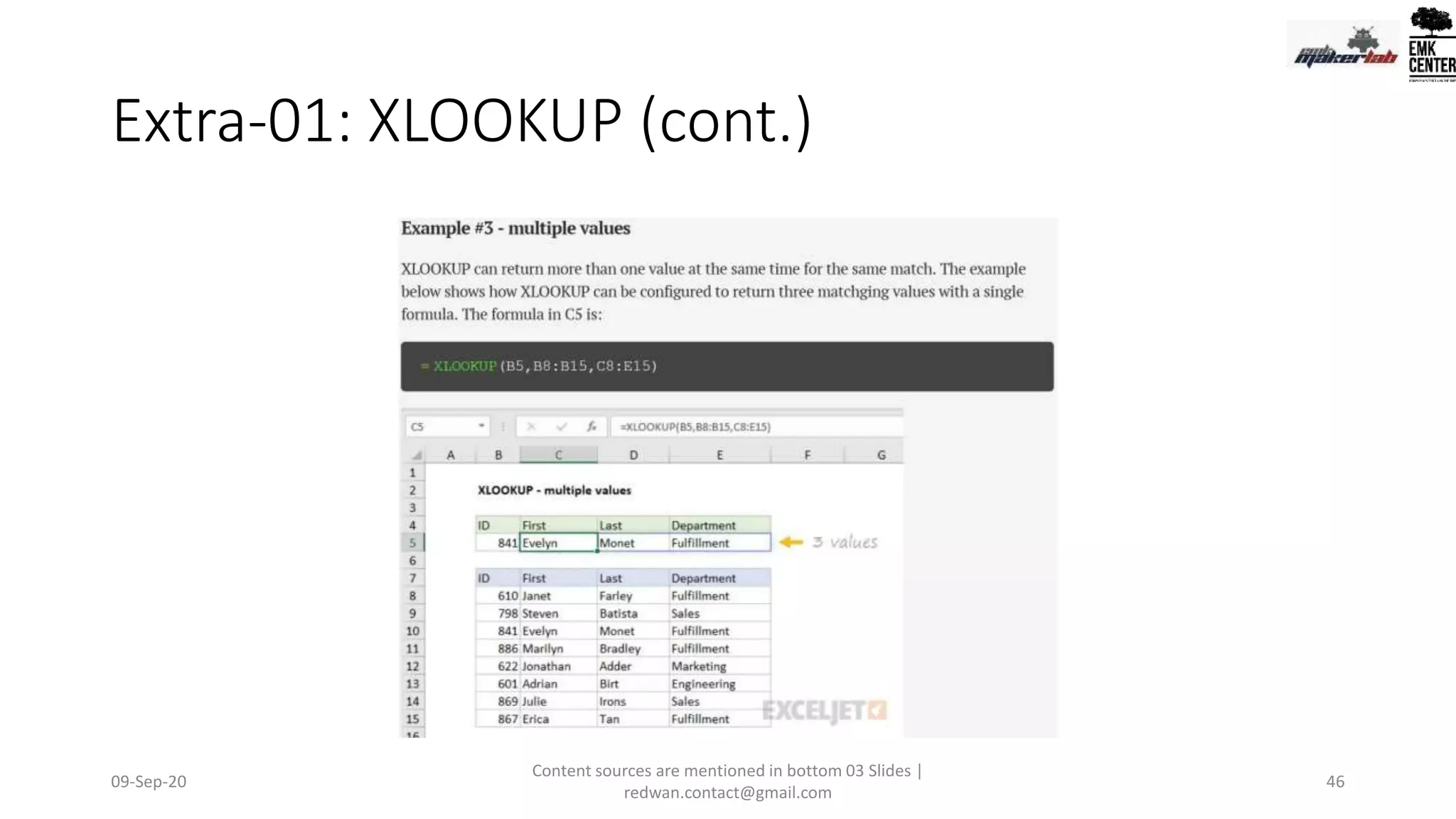
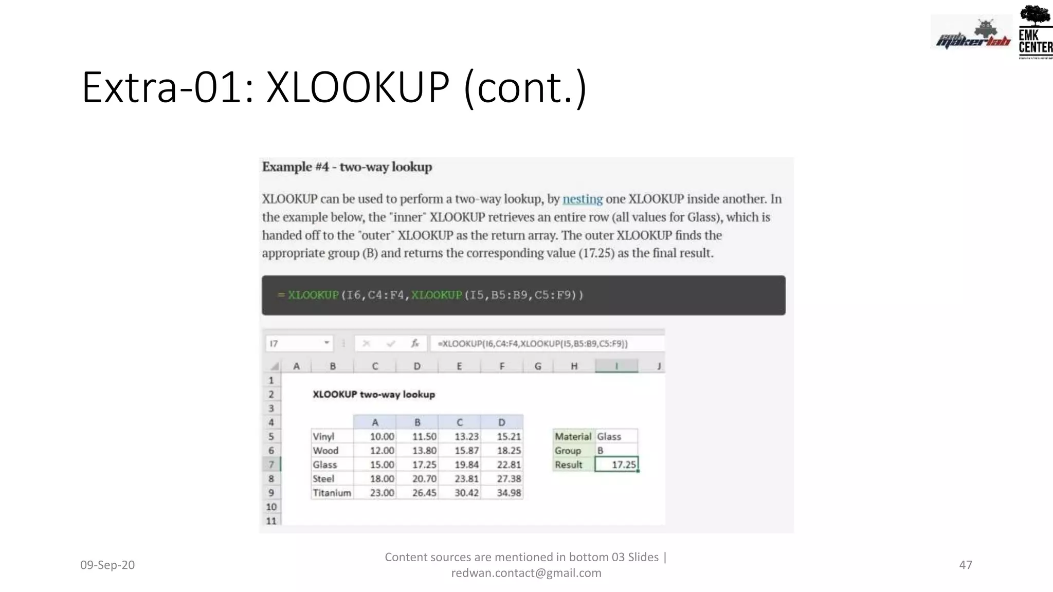
![Extra-01: XLOOKUP (cont.)
Arguments:
• lookup - The lookup value.
• lookup_array - The array or range to search.
• return_array - The array or range to return.
• not_found - [optional] Value to return if no match found.
• match_mode - [optional] 0 = exact match (default), -1 = exact match
or next smallest, 1 = exact match or next larger, 2 = wildcard match.
• search_mode - [optional] 1 = search from first (default), -1 = search
from last, 2 = binary search ascending, -2 = binary search descending.
09-Sep-20
Content sources are mentioned in bottom 03 Slides |
redwan.contact@gmail.com
41](https://image.slidesharecdn.com/basicdataanalysisforsmeusingmsexcelday-03-200910045123/75/Elementary-Data-Analysis-with-MS-Excel_Day-3-41-2048.jpg)
![Macro
• If you have tasks in Microsoft Excel that you do repeatedly, you can record a
macro to automate those tasks. Kind of Robotic Process Automation [RPA]
• A macro is an action or a set of actions that you can run as many times as you
want. When you create a macro, you are recording your mouse clicks and
keystrokes.
• After you create a macro, you can edit it to make minor changes to the way it
works.
• Suppose, that every month, you create a report for your accounting manager. You
want to format the names of the customers with overdue accounts in red, and
also apply bold formatting. You can create and then run a macro that quickly
applies these formatting changes to the cells you select.
09-Sep-20
Content sources are mentioned in bottom 03 Slides |
redwan.contact@gmail.com
75](https://image.slidesharecdn.com/basicdataanalysisforsmeusingmsexcelday-03-200910045123/75/Elementary-Data-Analysis-with-MS-Excel_Day-3-75-2048.jpg)


![Today’s Agenda
(IF, Nested IF, VLOOKUP, HLOOKUP)
- Formulas and Functions
- List of Formulas [Practical]
- 15 Important Functions for Data Analysis+ Practice
- Error Handling
- Data Validation
- Macro
09-Sep-20
Content sources are mentioned in bottom 03 Slides |
redwan.contact@gmail.com
2](https://crownmelresort.com/image.slidesharecdn.com/basicdataanalysisforsmeusingmsexcelday-03-200910045123/75/Elementary-Data-Analysis-with-MS-Excel_Day-3-2-2048.jpg)


![DAYS/NETWORKDAYS
• =DAYS is exactly what it implies. This function determines the number of calendar days between
two dates. This is a useful tool for assessing the lifecycle of products, contracts, and run rating
revenue depending on service length – a data analysis essential.
=NETWORKDAYS is slightly more robust and useful. This formula determines the number of
“workdays” between two dates as well as an option to account for holidays. Even workaholics
need a break now and then! Using these two formulas to compare time frames is especially
helpful for project management.
• Formulas:
=DAYS(SELECT CELL, SELECT CELL)
• OR
=NETWORKDAYS(SELECT CELL, SELECT CELL,[numberofholidays])
note: [numberofholidays] is optional
09-Sep-20
Content sources are mentioned in bottom 03 Slides |
redwan.contact@gmail.com
14](https://crownmelresort.com/image.slidesharecdn.com/basicdataanalysisforsmeusingmsexcelday-03-200910045123/75/Elementary-Data-Analysis-with-MS-Excel_Day-3-14-2048.jpg)

![SUMIFS
• =SUMIFS is one of the “must-know” formulas for a data analyst. The
common formula used is =SUM, but what if you need to sum values based
on multiple criteria? SUMIFS is it. In the example below, SUMIFS is used to
determine how much each product is contributing to top-line revenue.
• Formula:
=SUMIFS (sum_range, range1, criteria1, [range2], [criteria2], ...)
• example:
= SUMIFS(F5:F11,C5:C11,"red") // sum if red
= SUMIFS(F5:F11,C5:C11,"red",D5:D11,"TX") // sum if red and TX
09-Sep-20
Content sources are mentioned in bottom 03 Slides |
redwan.contact@gmail.com
16](https://crownmelresort.com/image.slidesharecdn.com/basicdataanalysisforsmeusingmsexcelday-03-200910045123/75/Elementary-Data-Analysis-with-MS-Excel_Day-3-16-2048.jpg)
![SUMIFS (cont.)
Arguments:
• sum_range - The range to be summed.
• range1 - The first range to evaluate.
• criteria1 - The criteria to use on range1.
• range2 - [optional] The second range to evaluate.
• criteria2 - [optional] The criteria to use on range2.
09-Sep-20
Content sources are mentioned in bottom 03 Slides |
redwan.contact@gmail.com
17](https://crownmelresort.com/image.slidesharecdn.com/basicdataanalysisforsmeusingmsexcelday-03-200910045123/75/Elementary-Data-Analysis-with-MS-Excel_Day-3-17-2048.jpg)

![AVERAGEIFS
• Much like SUMIFS, AVERAGEIFS allows you to take an average based
on one or more criteria.
Formula:
• =AVERAGEIF(SELECT CELL, CRITERIA,[AVERAGE_RANGE])
• note: [average_range] is optional
• example:
• =AVERAGEIF($C:$C,$A:$A,$F2)
09-Sep-20
Content sources are mentioned in bottom 03 Slides |
redwan.contact@gmail.com
19](https://crownmelresort.com/image.slidesharecdn.com/basicdataanalysisforsmeusingmsexcelday-03-200910045123/75/Elementary-Data-Analysis-with-MS-Excel_Day-3-19-2048.jpg)
![VLOOKUP
• VLOOKUP is one of the most useful and recognizable data analysis
functions. As an Excel user, you’ll probably need to “marry” data together
at some point. For example, accounts receivable might know how much
each product costs, but the shipping department can only provide units
shipped. This is the perfect use case for VLOOKUP.
Formula:
• =VLOOKUP(LOOKUP_VALUE,TABLE_ARRAY,COL_INDEX_NUM,
[RANGE_LOOKUP])
• example:
• =VLOOKUP(A5,$A$1:$G$44,3)
09-Sep-20
Content sources are mentioned in bottom 03 Slides |
redwan.contact@gmail.com
20](https://crownmelresort.com/image.slidesharecdn.com/basicdataanalysisforsmeusingmsexcelday-03-200910045123/75/Elementary-Data-Analysis-with-MS-Excel_Day-3-20-2048.jpg)


![FIND/SEARCH
• =FIND/=SEARCH are powerful functions for isolating specific text within a data
set. Both are listed here because =FIND will return a case-sensitive match, i.e. if
you use FIND to query for “Big” you will only return Big=true results. But a
=SEARCH for “Big” will match with Big or big, making the query a bit broader. This
is particularly useful for looking for anomalies or unique identifiers.
Formula:
• =FIND(TEXT,WITHIN_TEXT,[START_NUMBER]) OR
=SEARCH(TEXT,WITHIN_TEXT,[START_NUMBER])
• note: [start_number] is optional and is used to indicate the starting cell in the text
to search
• example:
• =(FIND(“Central”, B2))
09-Sep-20
Content sources are mentioned in bottom 03 Slides |
redwan.contact@gmail.com
24](https://crownmelresort.com/image.slidesharecdn.com/basicdataanalysisforsmeusingmsexcelday-03-200910045123/75/Elementary-Data-Analysis-with-MS-Excel_Day-3-24-2048.jpg)


![RANK
• =RANK is an ancient excel function, but that doesn’t downplay its
effectiveness for data analysis. =RANK allows you to quickly denote how
values rank in a dataset in ascending or descending order. In the example,
RANK is being used to determine which clients order the most product.
Formula:
• =RANK(SELECT CELL,RANGE_TO_RANK_AGAINST,[ORDER])
• note: [order] is optional
• example:
• =RANK(H1,$H$1:$H$43)
09-Sep-20
Content sources are mentioned in bottom 03 Slides |
redwan.contact@gmail.com
32](https://crownmelresort.com/image.slidesharecdn.com/basicdataanalysisforsmeusingmsexcelday-03-200910045123/75/Elementary-Data-Analysis-with-MS-Excel_Day-3-32-2048.jpg)


![Extra-01: XLOOKUP (Office365)
• The Excel XLOOKUP function is a modern and flexible replacement for
older functions like VLOOKUP, HLOOKUP, and LOOKUP. XLOOKUP
supports approximate and exact matching, wildcards (* ?) for partial
matches, and lookups in vertical or horizontal ranges.
• Syntax
=XLOOKUP (lookup, lookup_array, return_array, [not_found],
[match_mode], [search_mode])
09-Sep-20
Content sources are mentioned in bottom 03 Slides |
redwan.contact@gmail.com
40](https://crownmelresort.com/image.slidesharecdn.com/basicdataanalysisforsmeusingmsexcelday-03-200910045123/75/Elementary-Data-Analysis-with-MS-Excel_Day-3-40-2048.jpg)
![Extra-01: XLOOKUP (cont.)
Arguments:
• lookup - The lookup value.
• lookup_array - The array or range to search.
• return_array - The array or range to return.
• not_found - [optional] Value to return if no match found.
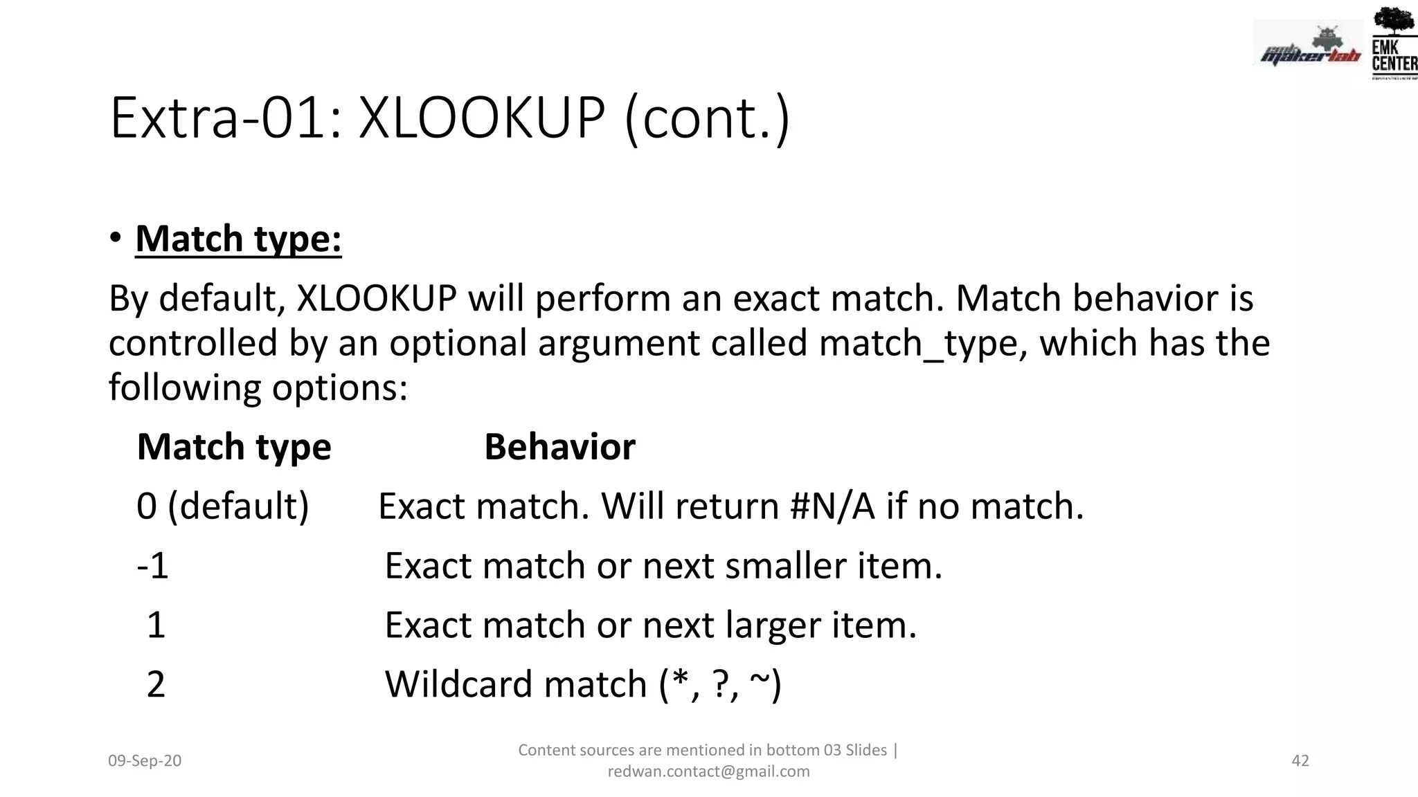
• match_mode - [optional] 0 = exact match (default), -1 = exact match
or next smallest, 1 = exact match or next larger, 2 = wildcard match.
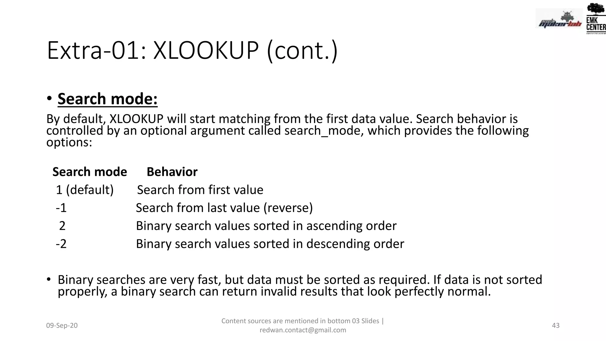
• search_mode - [optional] 1 = search from first (default), -1 = search
from last, 2 = binary search ascending, -2 = binary search descending.
09-Sep-20
Content sources are mentioned in bottom 03 Slides |
redwan.contact@gmail.com
41](https://crownmelresort.com/image.slidesharecdn.com/basicdataanalysisforsmeusingmsexcelday-03-200910045123/75/Elementary-Data-Analysis-with-MS-Excel_Day-3-41-2048.jpg)


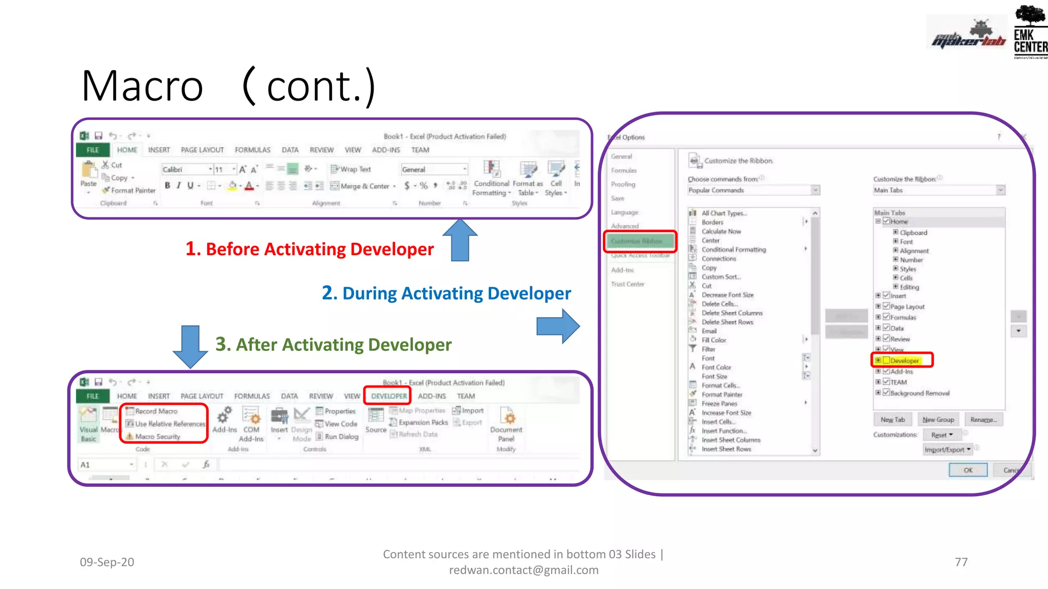
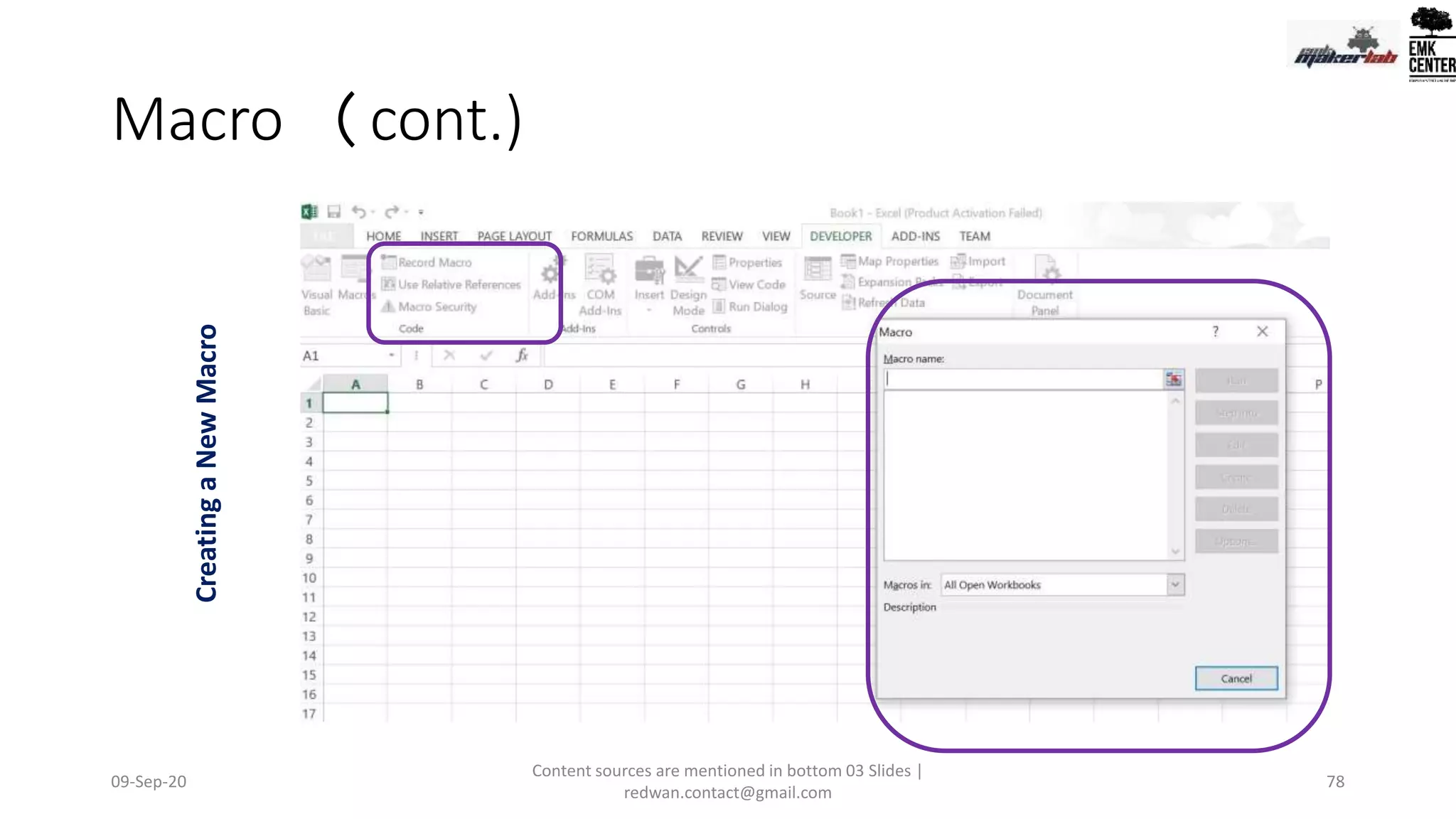
![Macro
• If you have tasks in Microsoft Excel that you do repeatedly, you can record a
macro to automate those tasks. Kind of Robotic Process Automation [RPA]
• A macro is an action or a set of actions that you can run as many times as you
want. When you create a macro, you are recording your mouse clicks and
keystrokes.
• After you create a macro, you can edit it to make minor changes to the way it
works.
• Suppose, that every month, you create a report for your accounting manager. You
want to format the names of the customers with overdue accounts in red, and
also apply bold formatting. You can create and then run a macro that quickly
applies these formatting changes to the cells you select.
09-Sep-20
Content sources are mentioned in bottom 03 Slides |
redwan.contact@gmail.com
75](https://crownmelresort.com/image.slidesharecdn.com/basicdataanalysisforsmeusingmsexcelday-03-200910045123/75/Elementary-Data-Analysis-with-MS-Excel_Day-3-75-2048.jpg)


The document provides an overview of essential Excel functions and formulas for performing elementary data analysis, including how to use formulas like SUMIF, VLOOKUP, and AVERAGEIF. It emphasizes important functions, practical applications, and provides examples to aid understanding. Additionally, it includes tips for error handling and keyboard shortcuts for efficiency in Excel operations.
Introduction to data analysis concepts using MS Excel, presented by Redwan Ferdous, with agenda including formulas and functions.
Explanation of formulas (custom calculations) and functions (predefined calculations) in Excel, along with a list of essential functions.
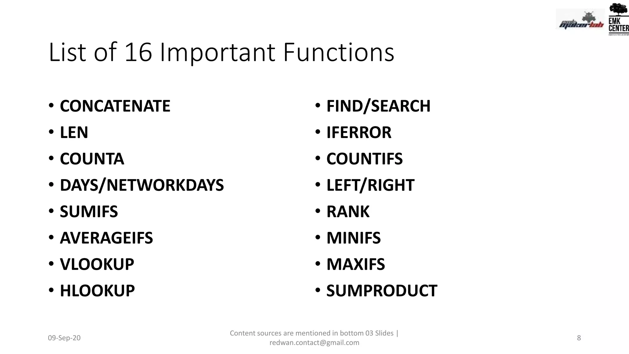
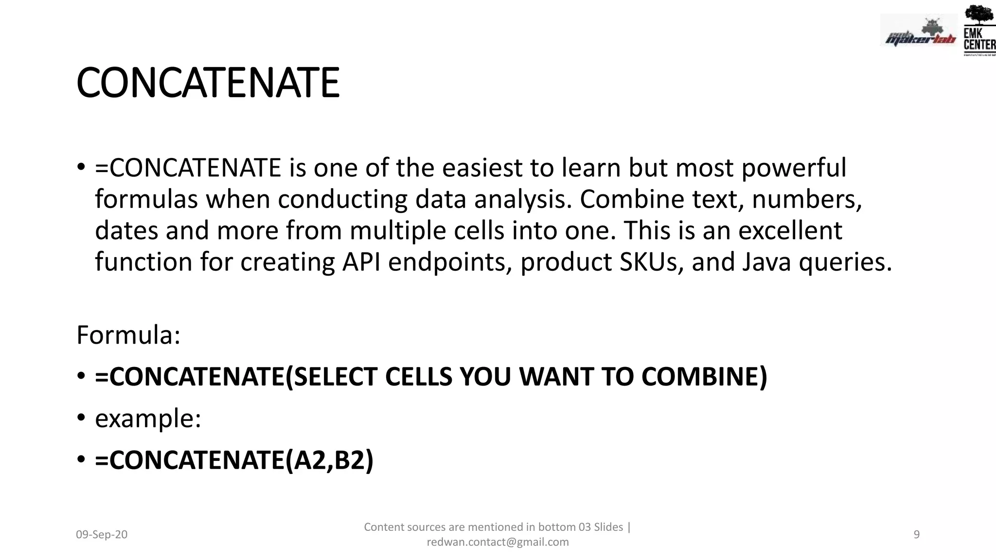
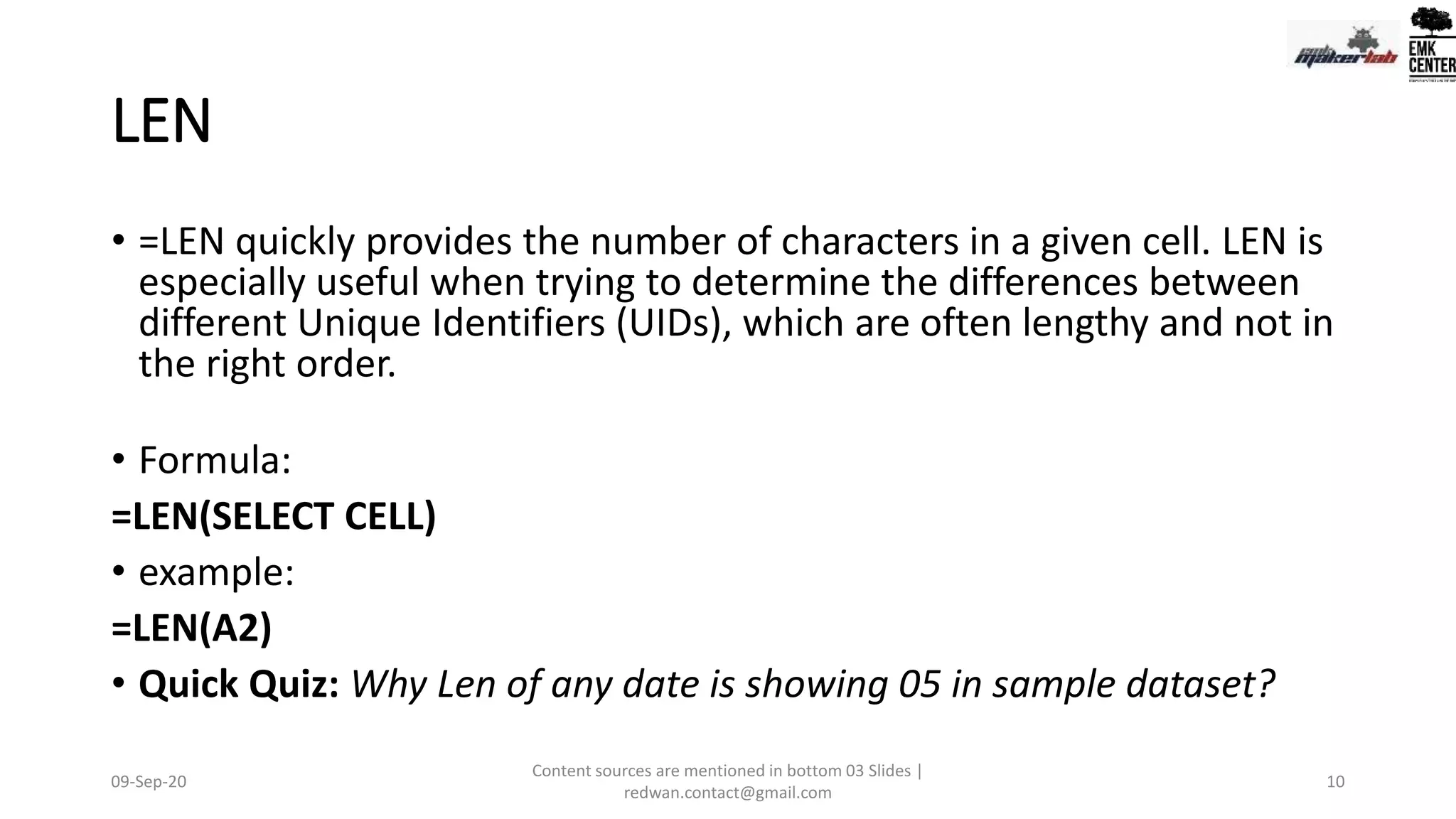
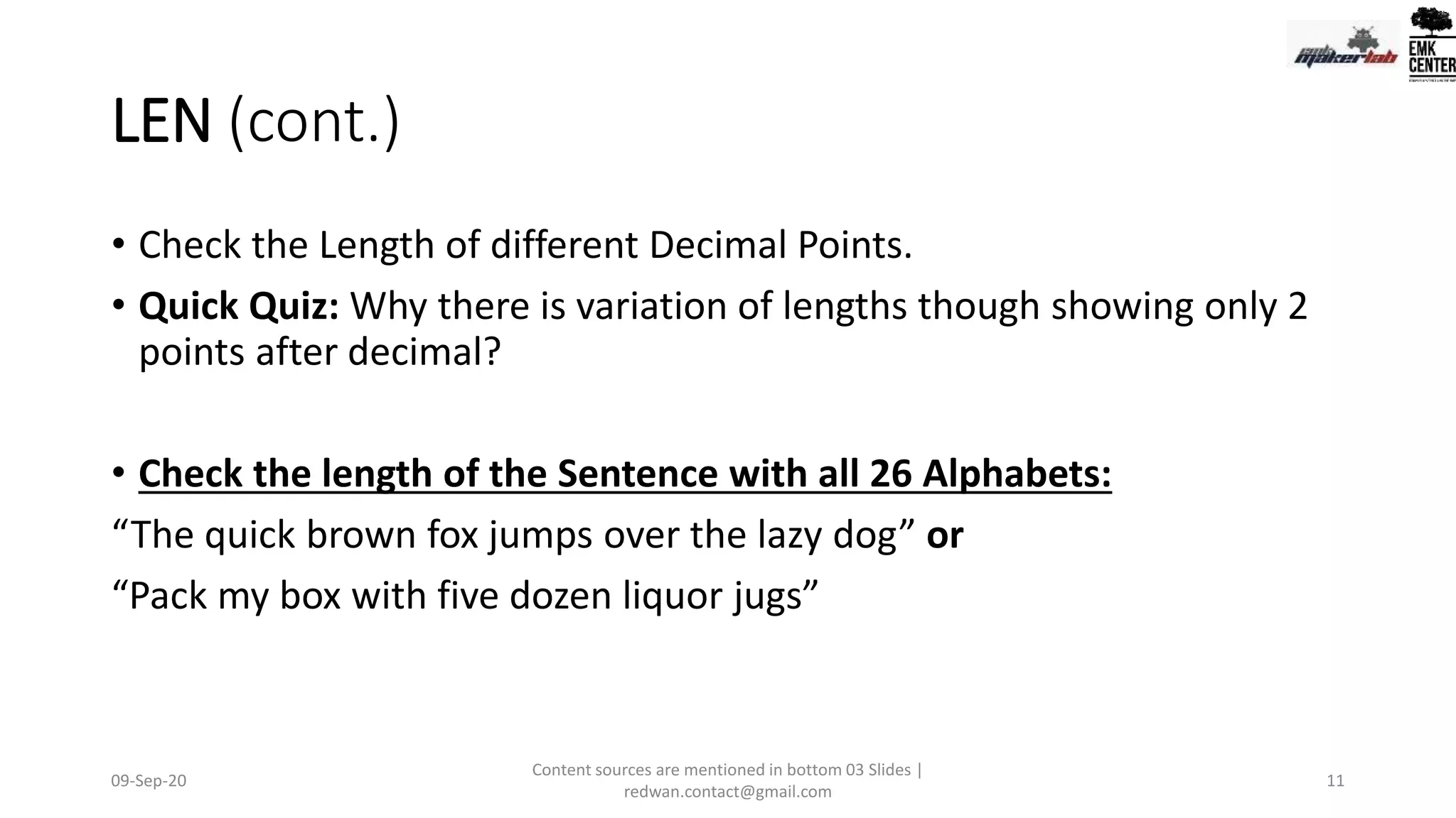
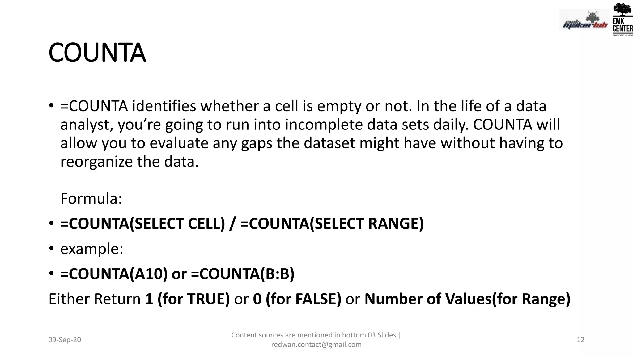
Detailed explanations of key functions like CONCATENATE, LEN, COUNTA, DAYS, NETWORKDAYS for effective data analysis.
Highlights of functions like SUMIFS, VLOOKUP, and HLOOKUP for conditional summation and lookups in data sets.
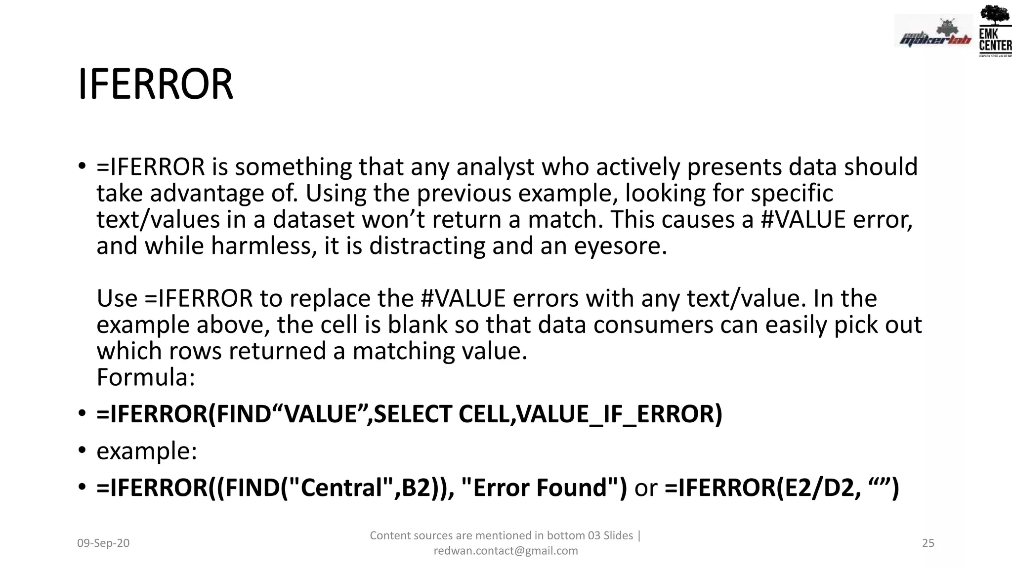
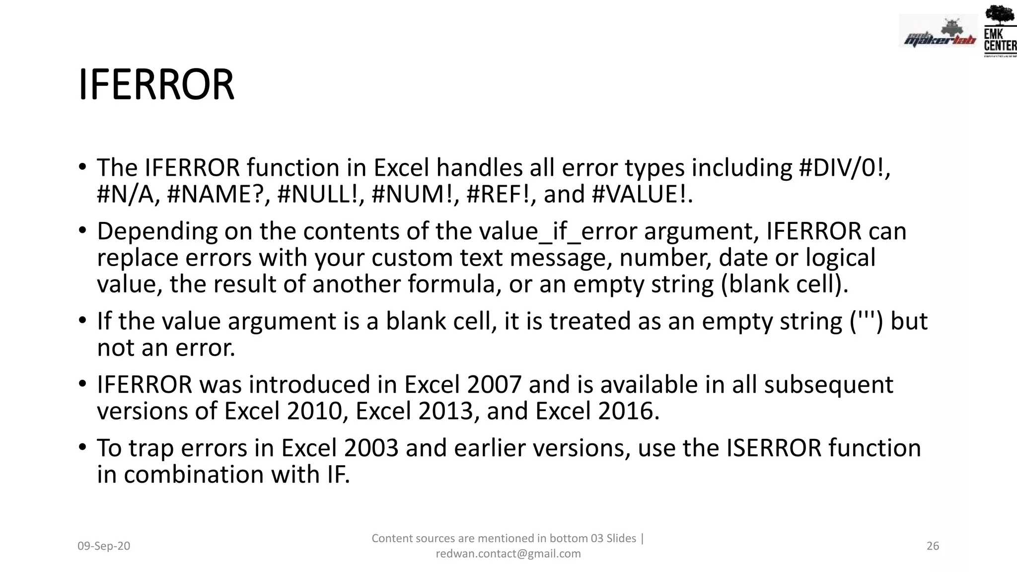
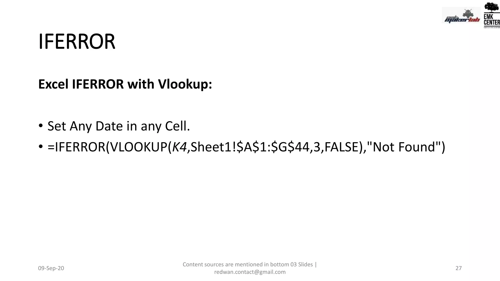
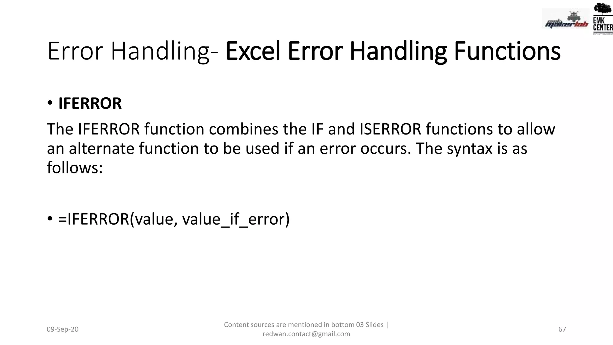
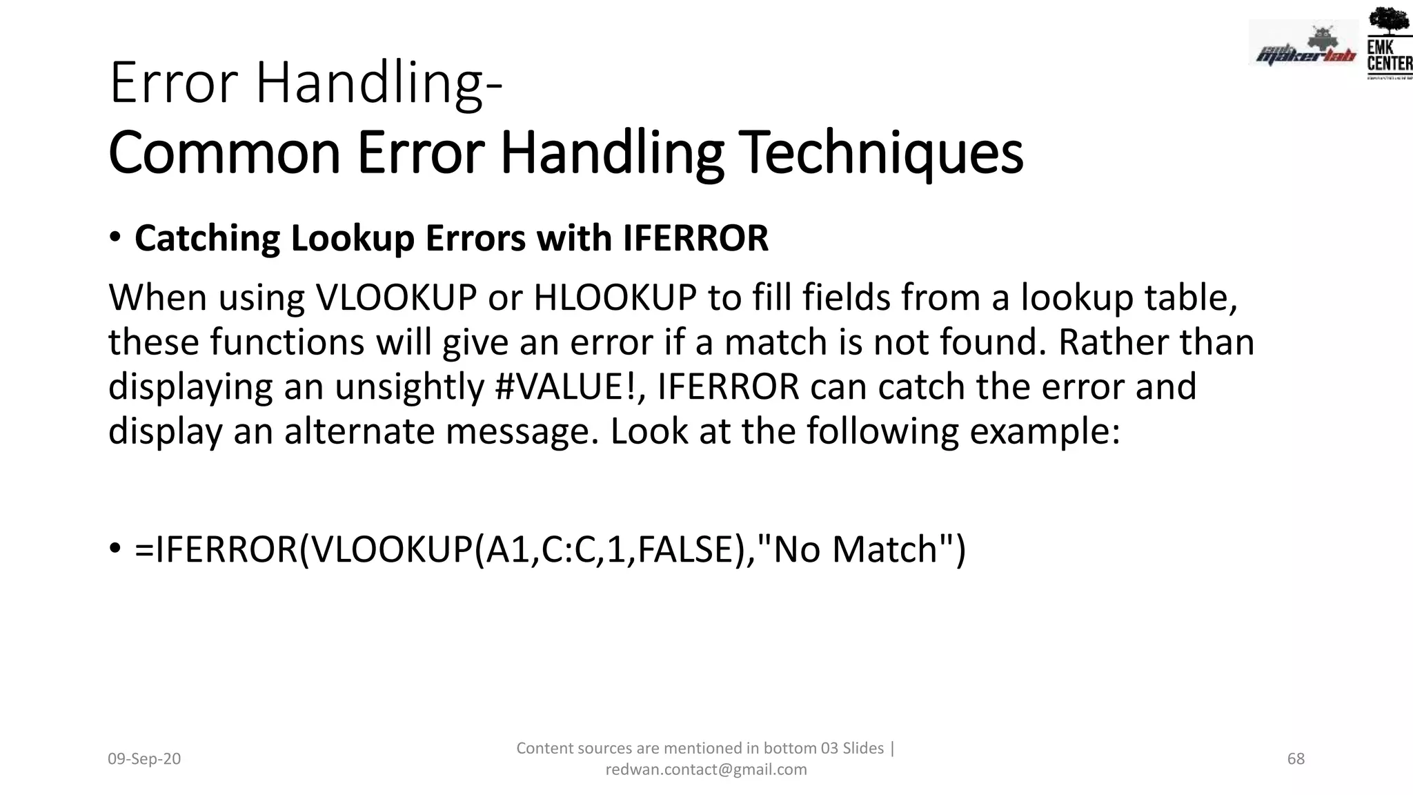
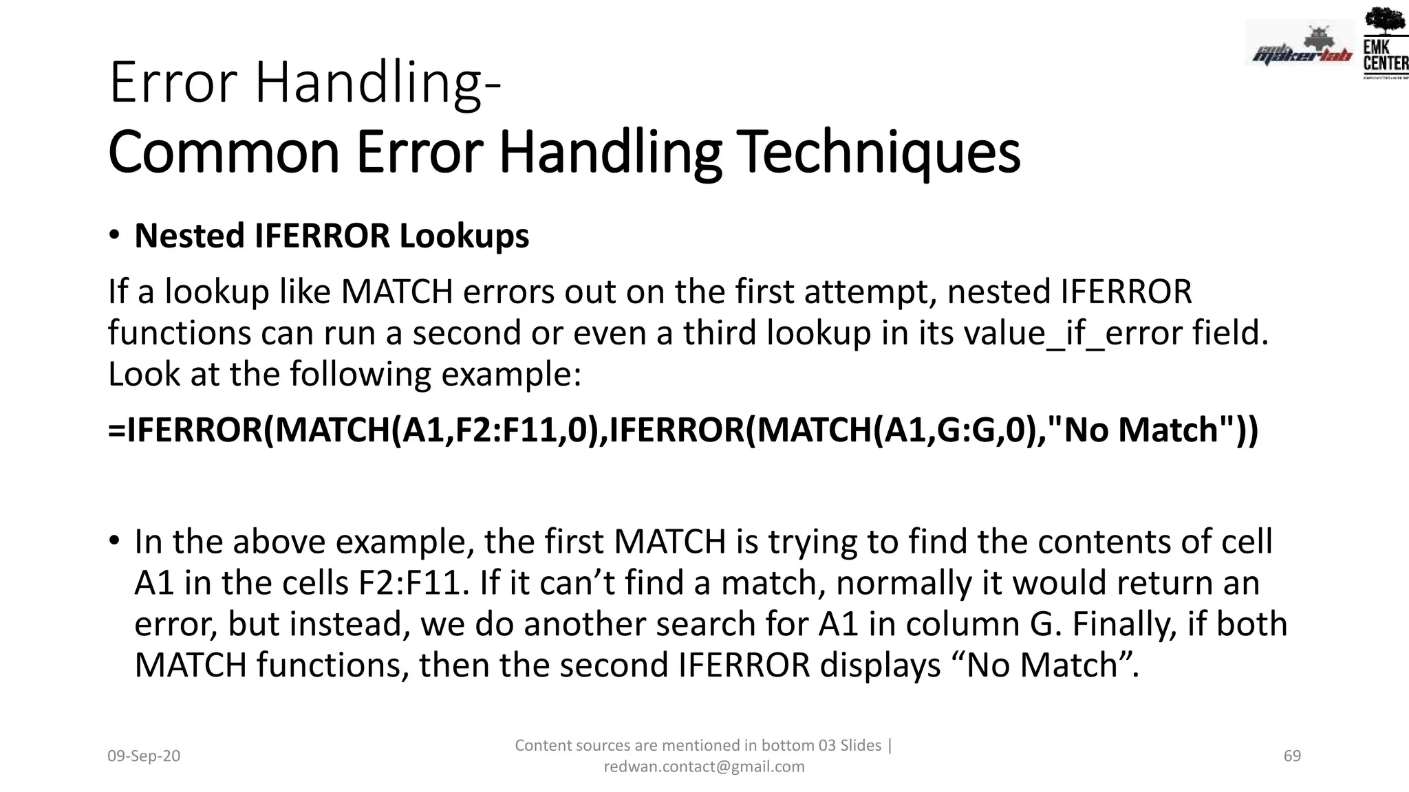
Introduction to error handling using IFERROR to manage errors in formulas, enhancing presentation of data.
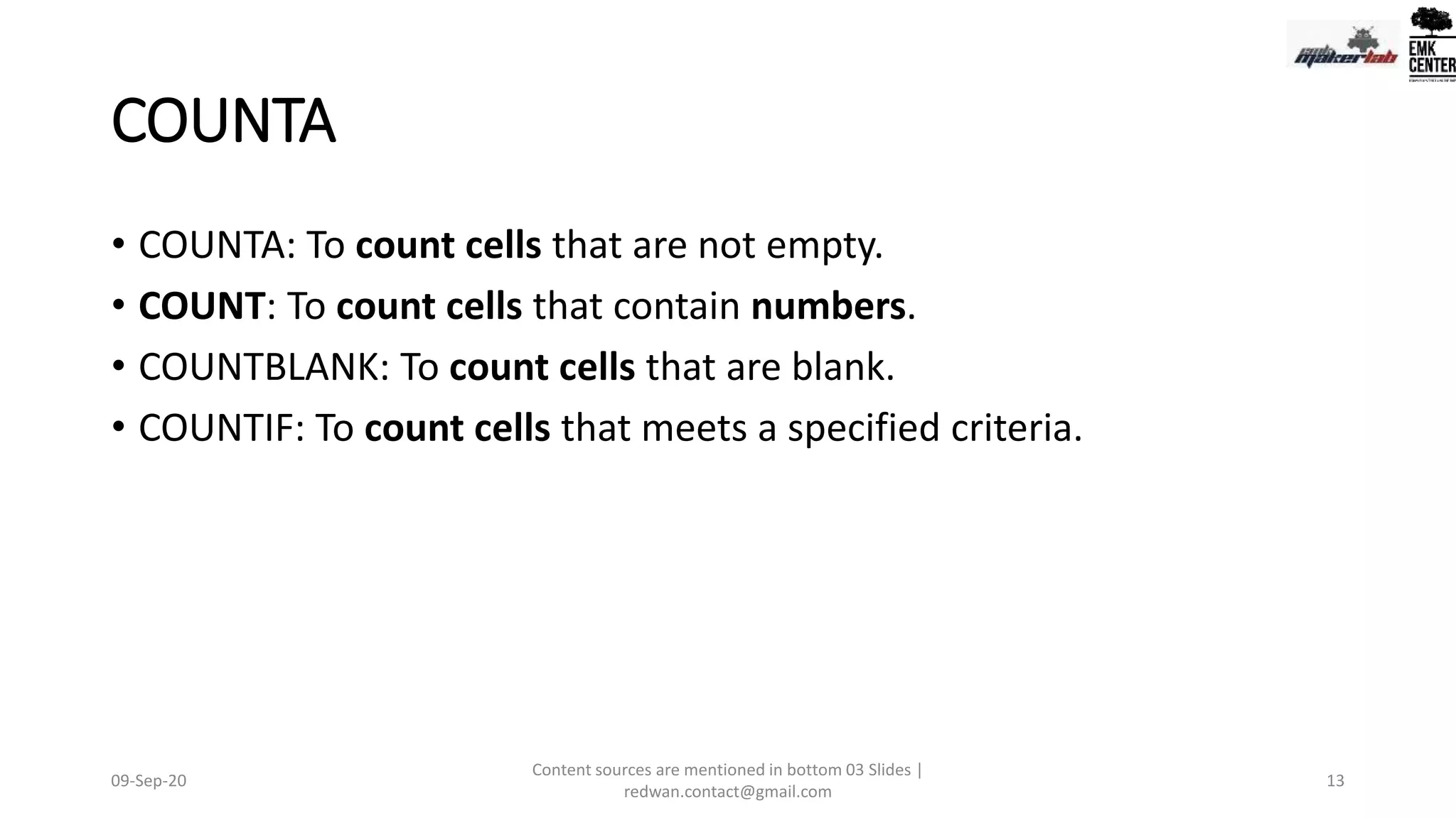
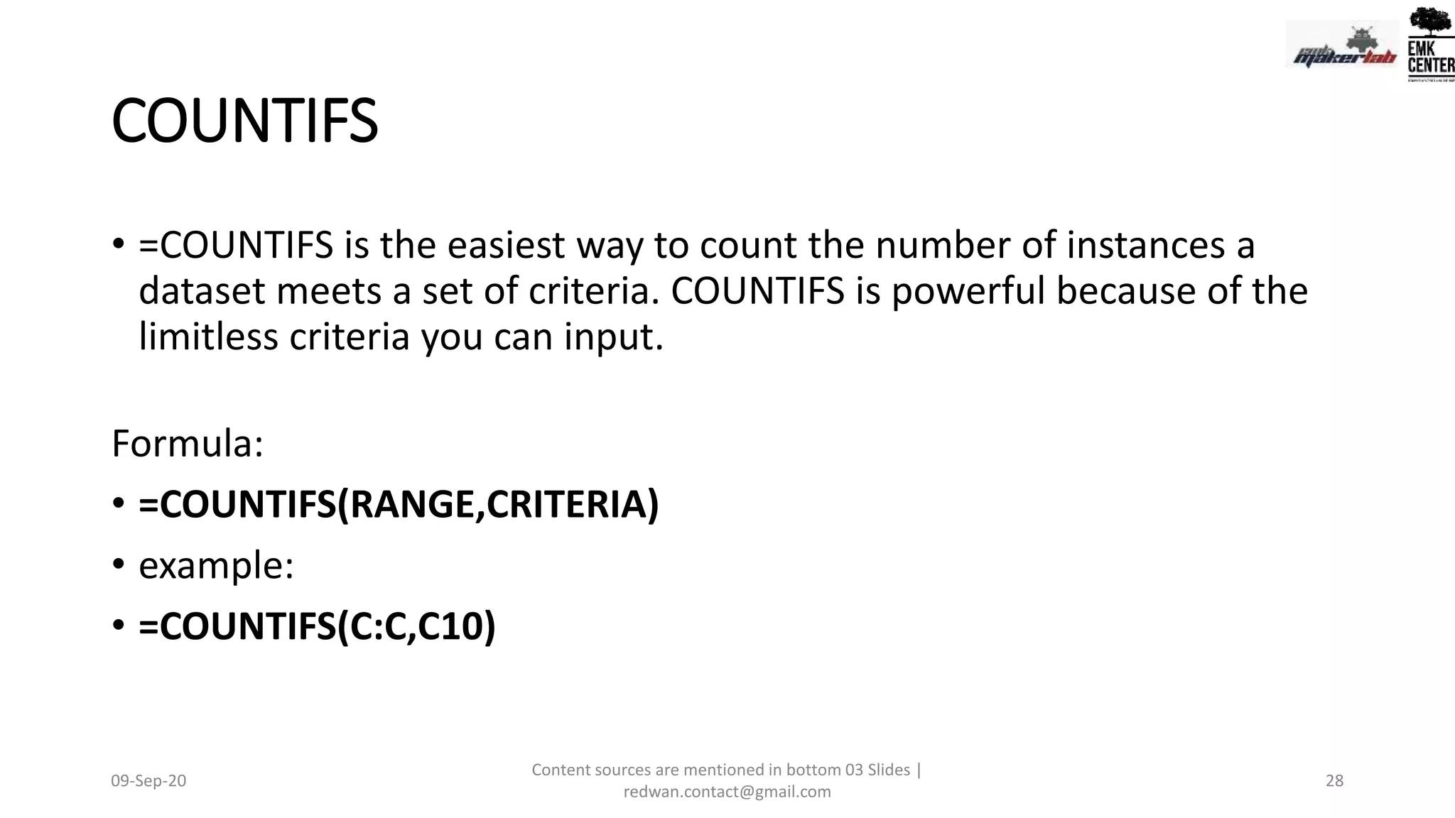
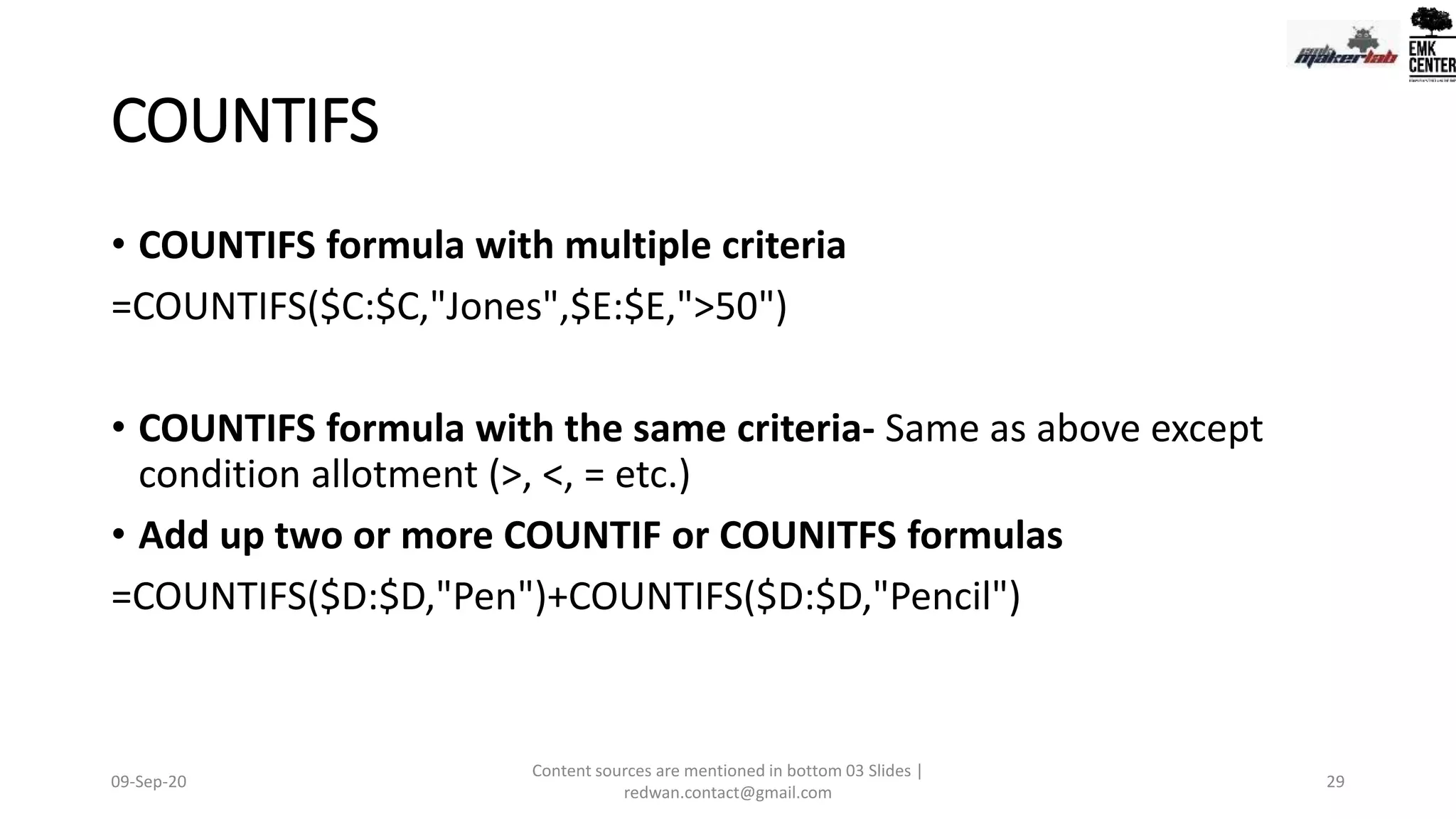
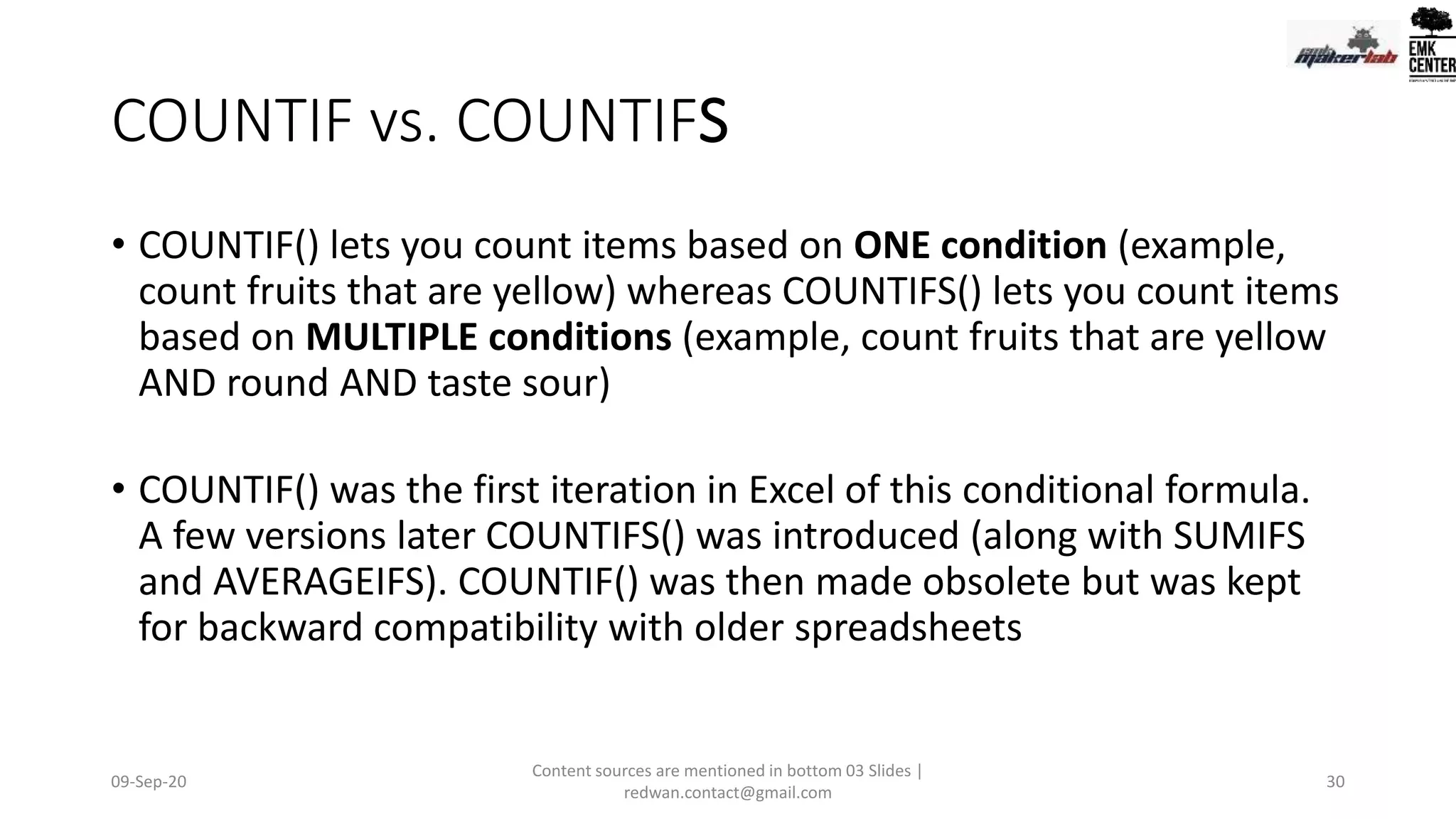
Differences between COUNTIF and COUNTIFS functions for counting criteria matches across datasets.
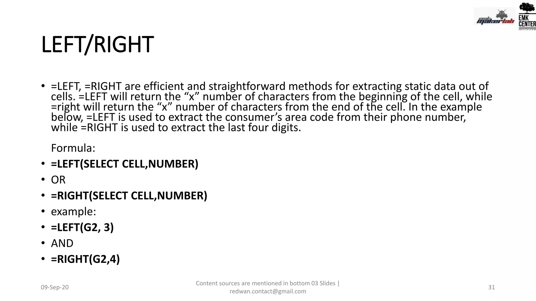
Using LEFT/RIGHT functions for text extraction and RANK function for ordering datasets based on values.
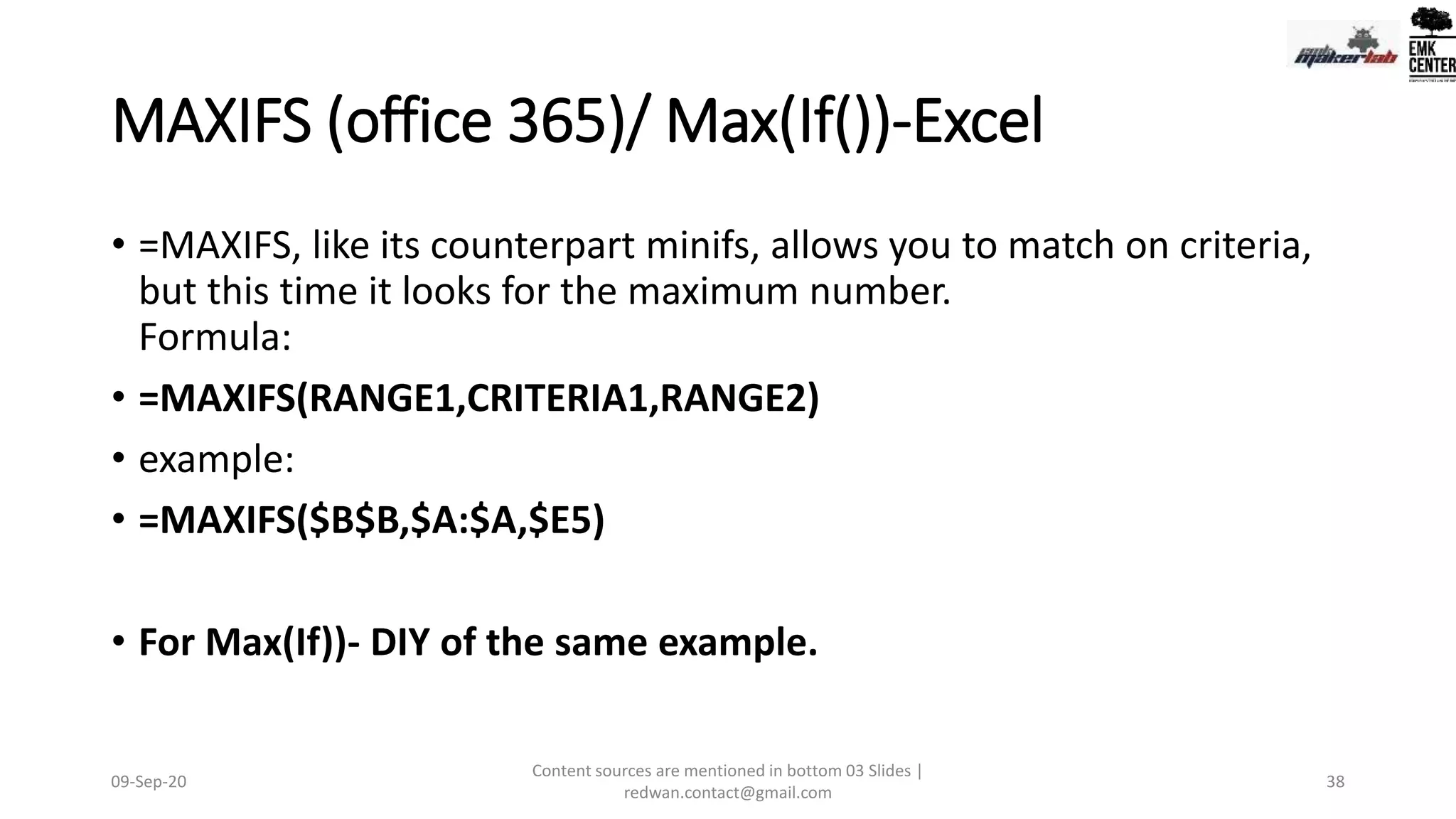
Overview of MINIFS and MAXIFS functions for conditional minimum and maximum calculations within datasets.
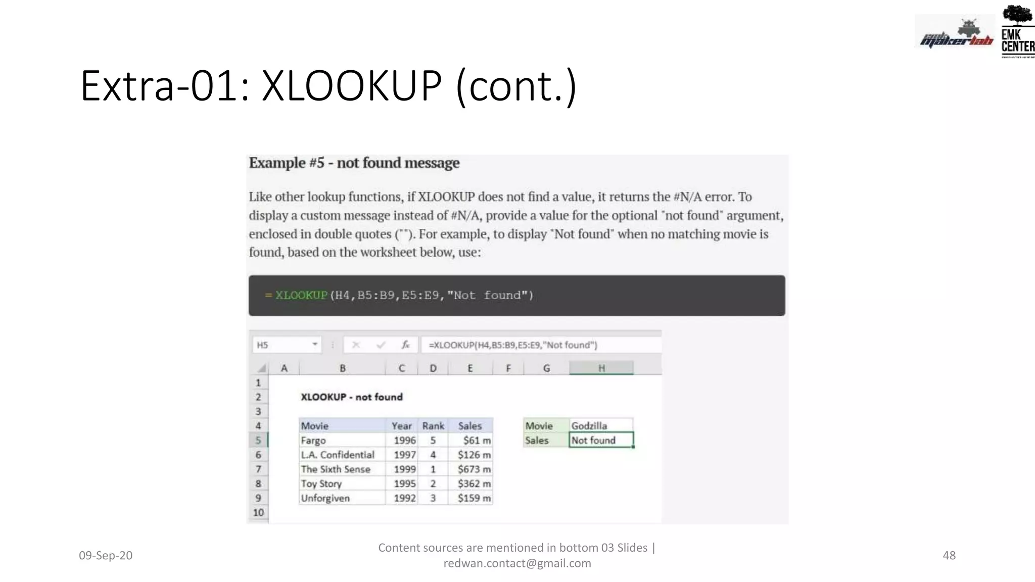
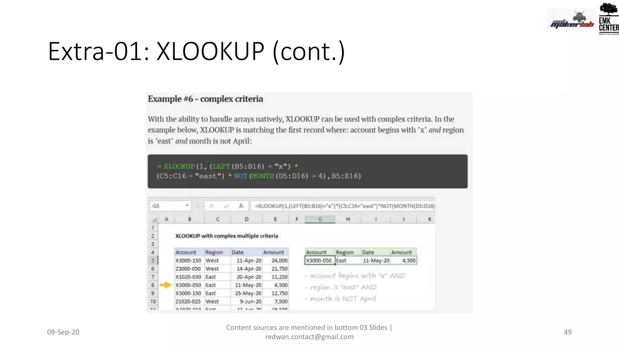
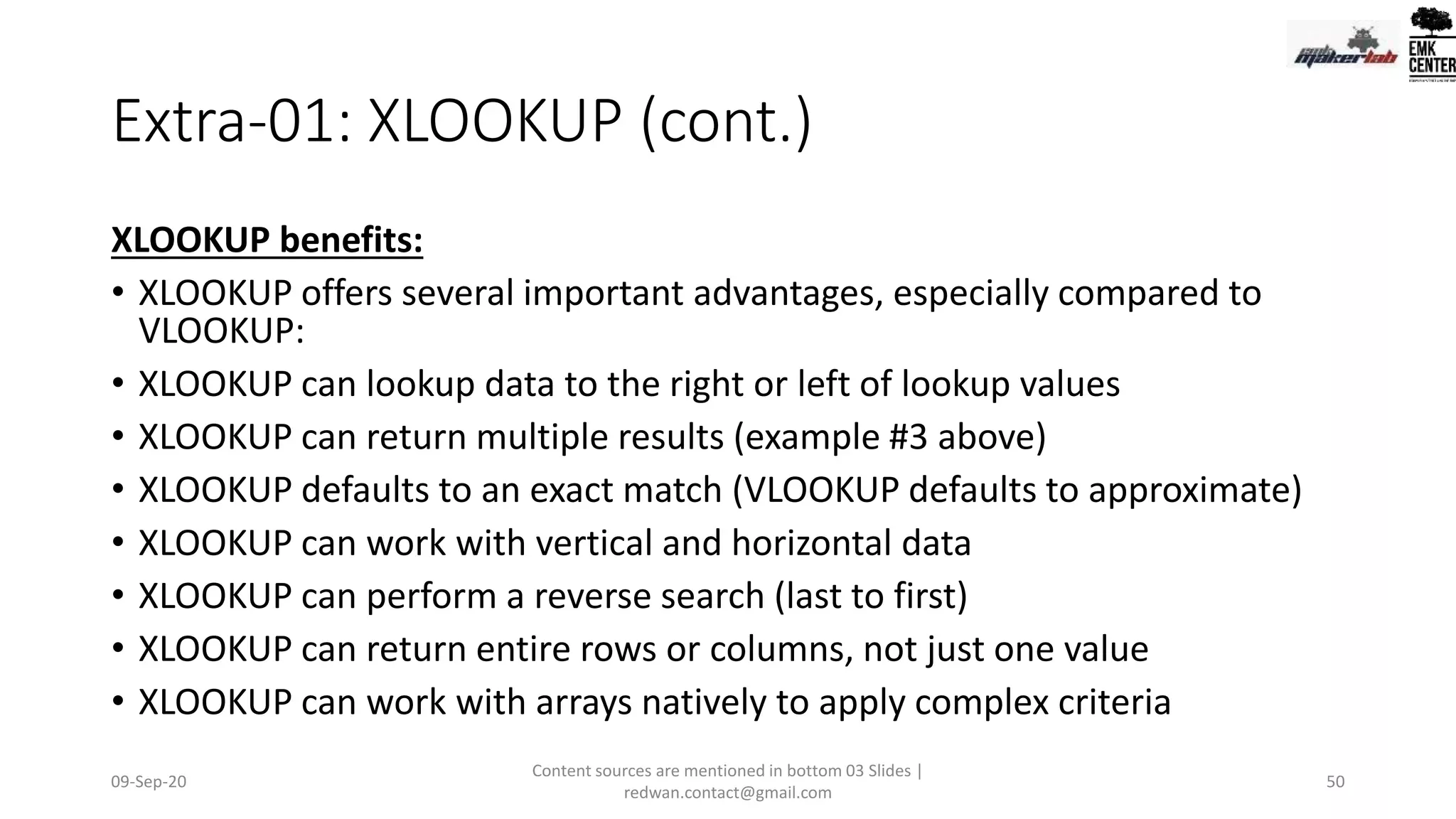
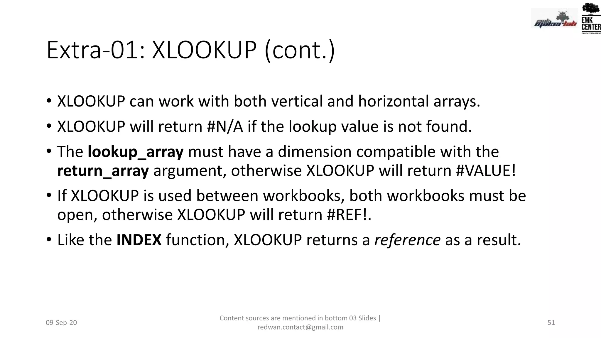
Introduction to XLOOKUP as a versatile replacement for VLOOKUP/HLOOKUP with advanced matching capabilities.
Usage of LOWER, UPPER, PROPER, and TRIM functions to standardize and clean text data in Excel.
Discussion on the IF function for conditional logic as a key tool in data analysis.
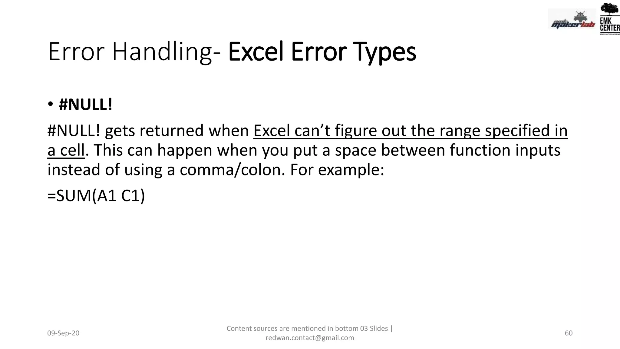
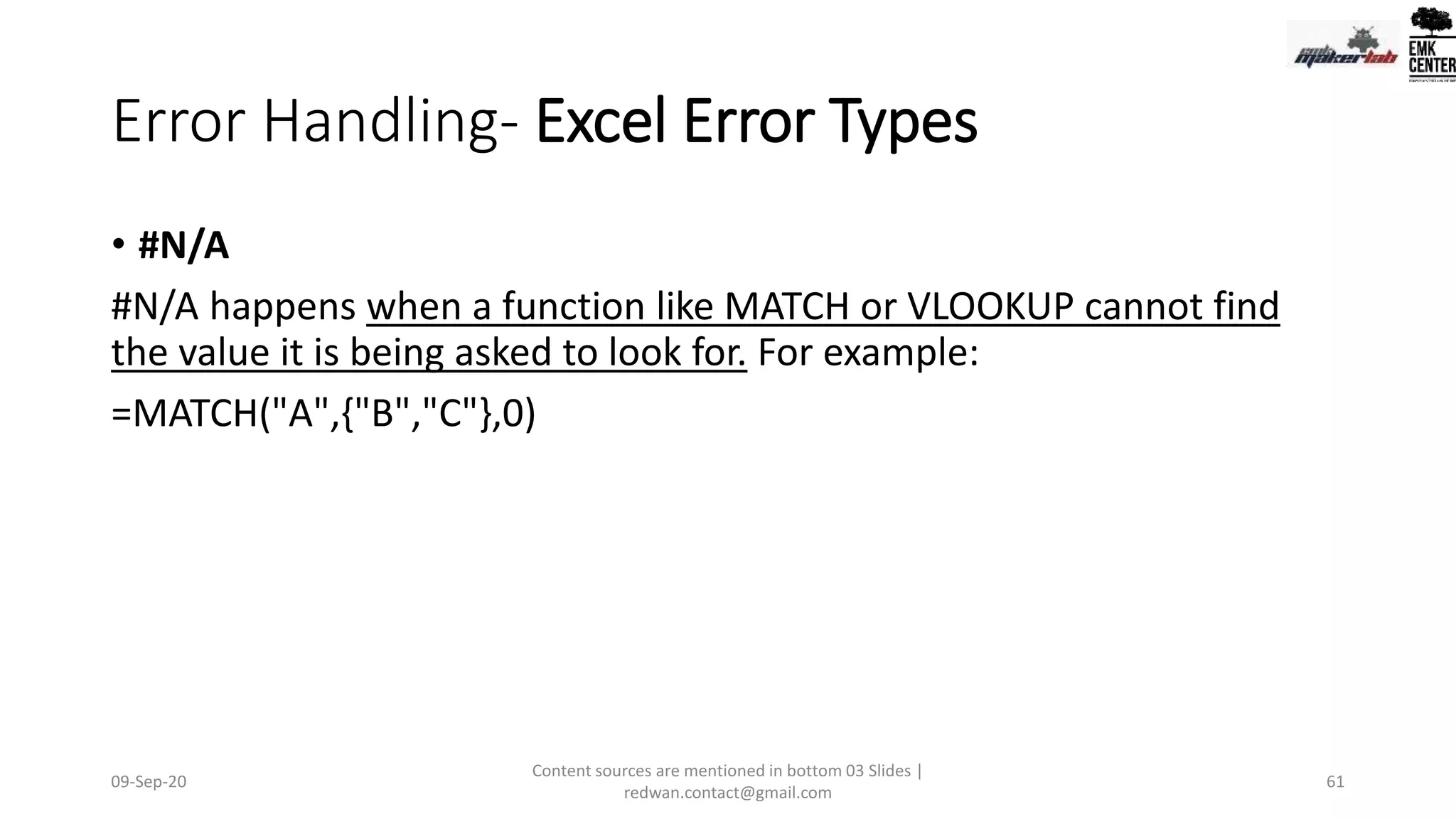
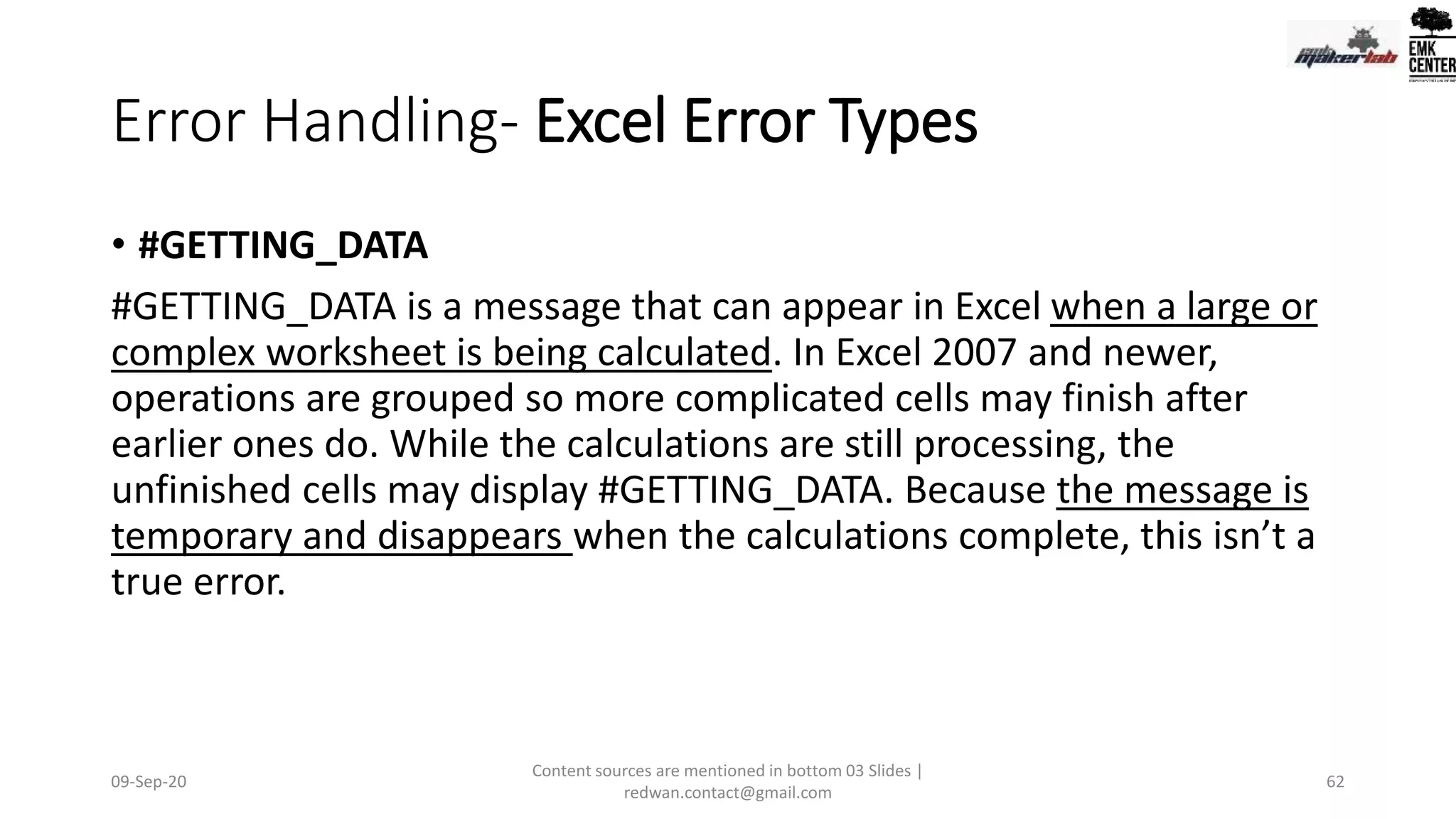
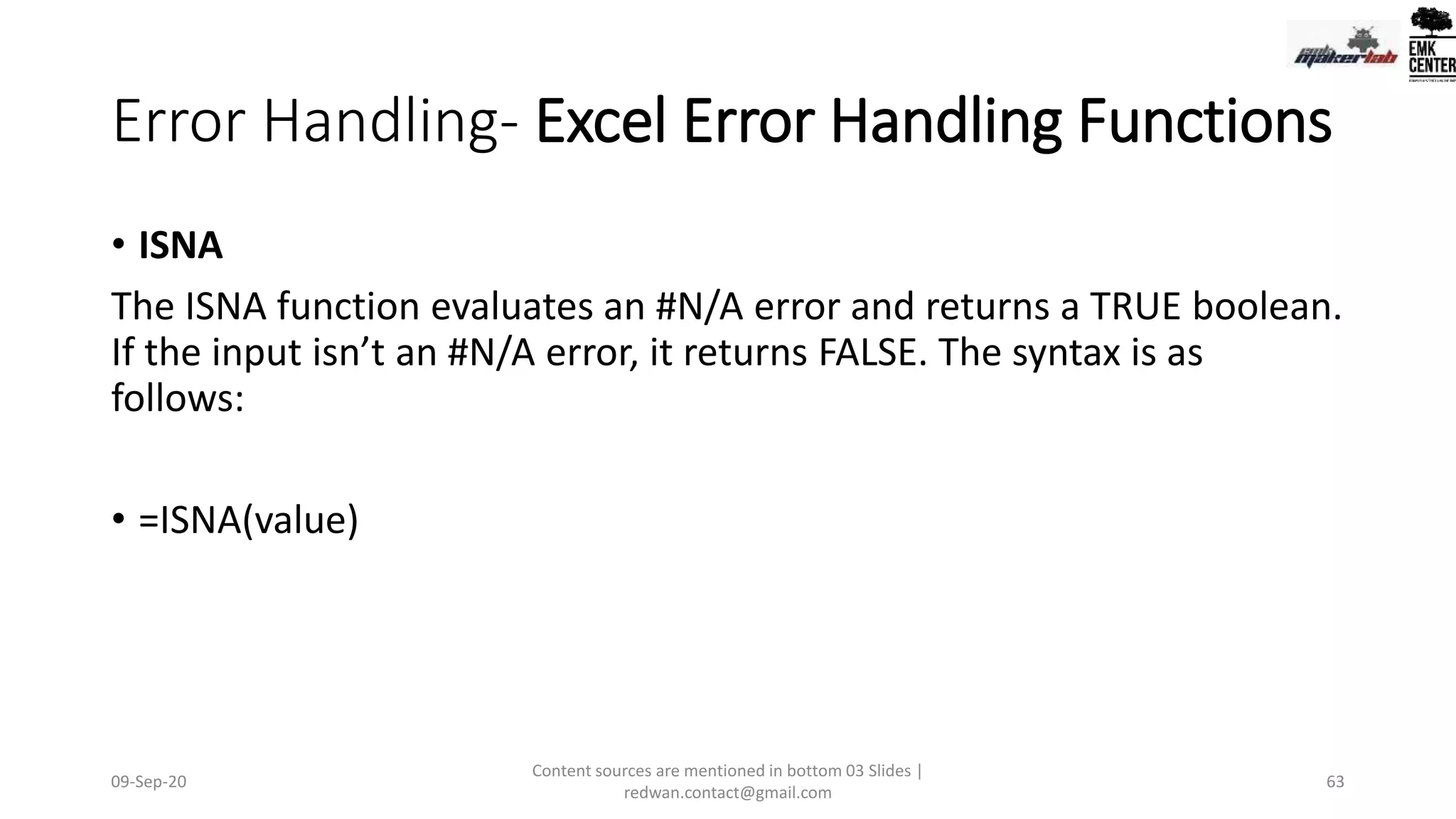
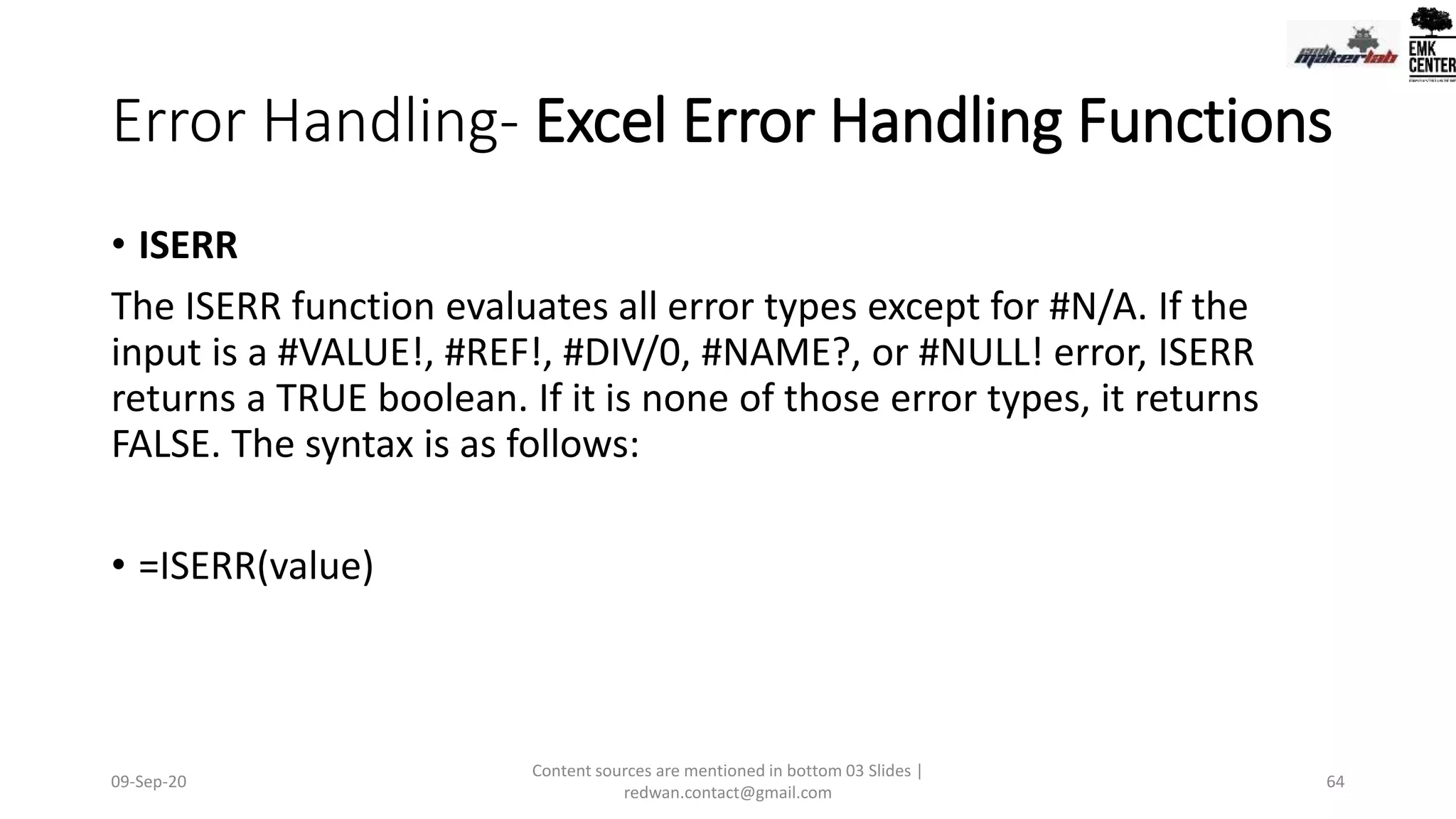
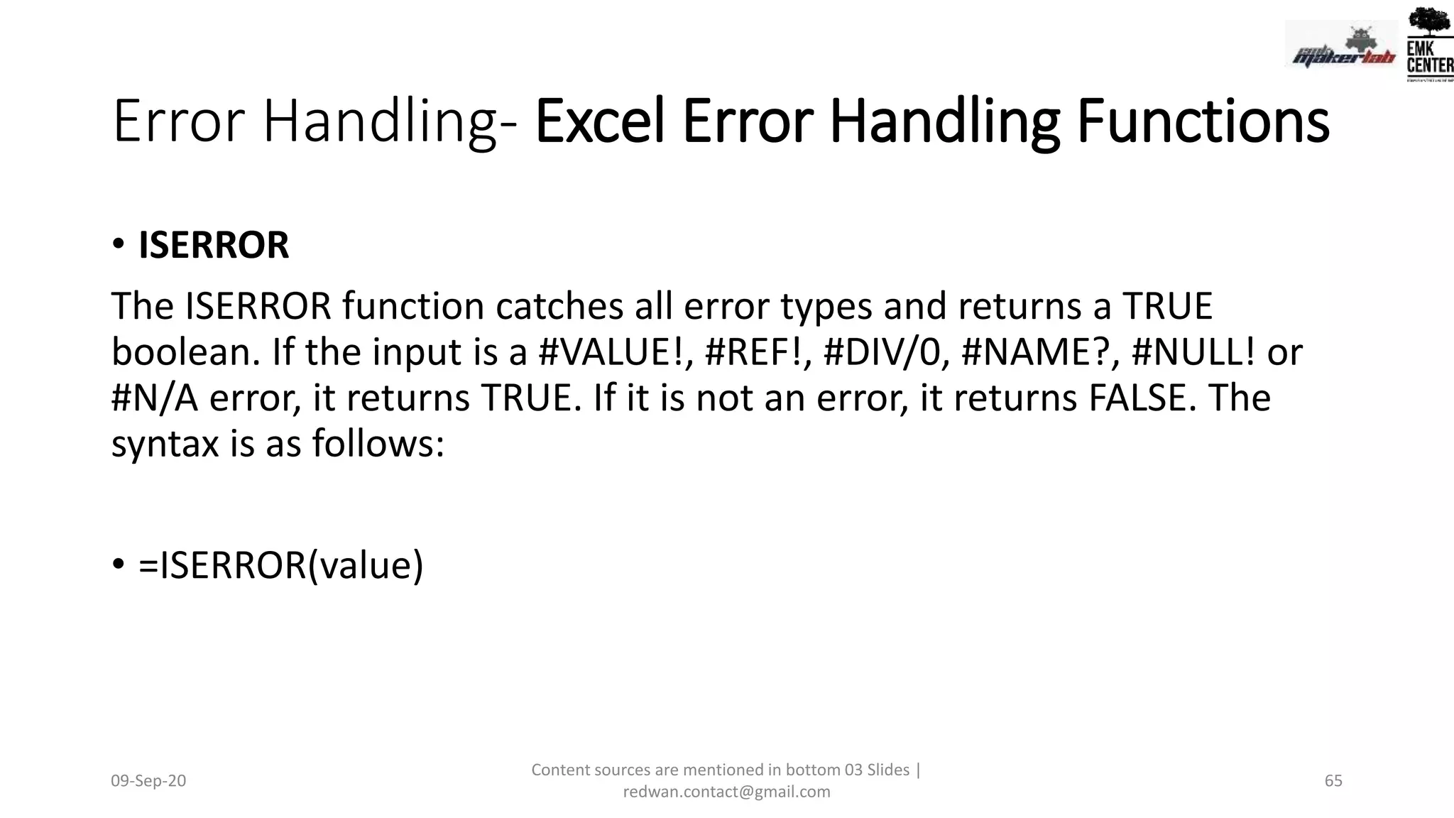
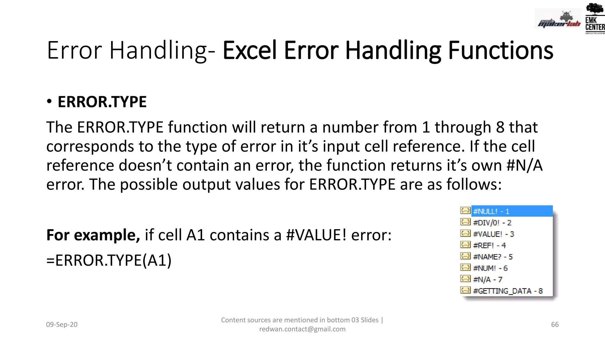
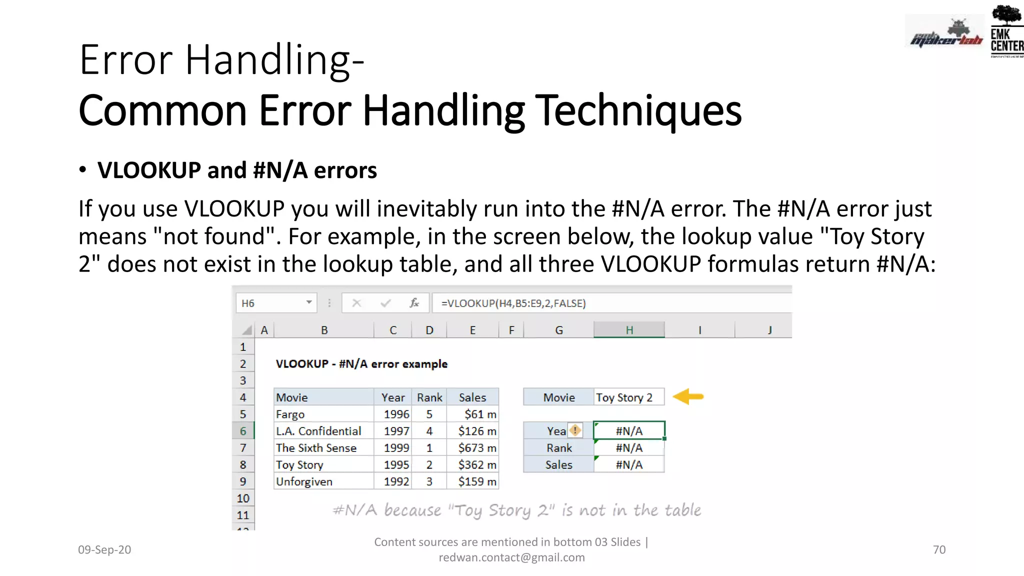
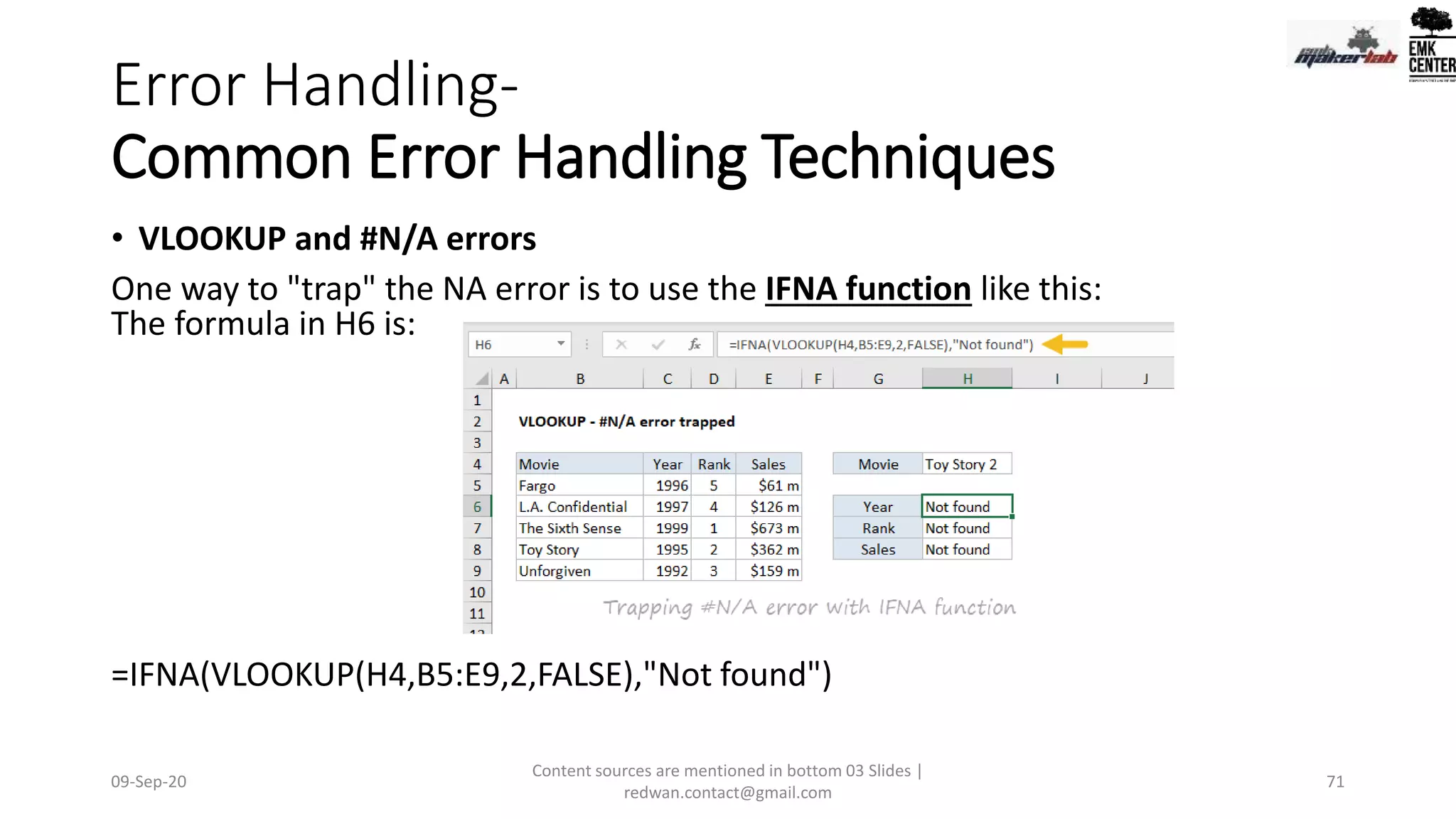
Various error types in Excel and effective handling strategies to prevent disruption in data analysis.
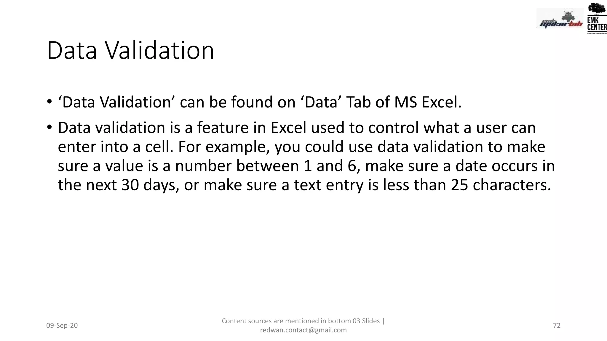
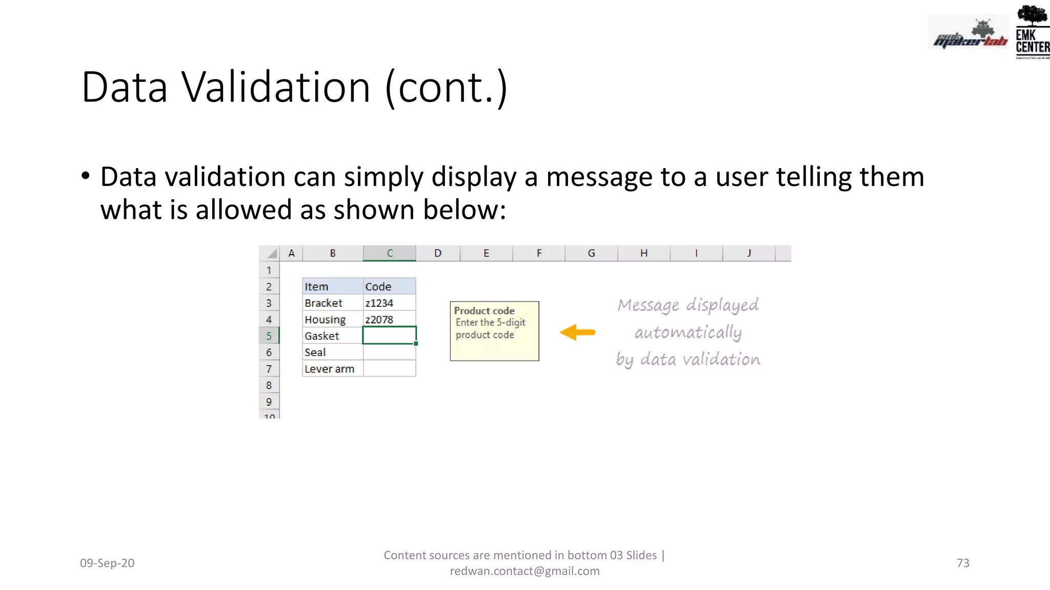
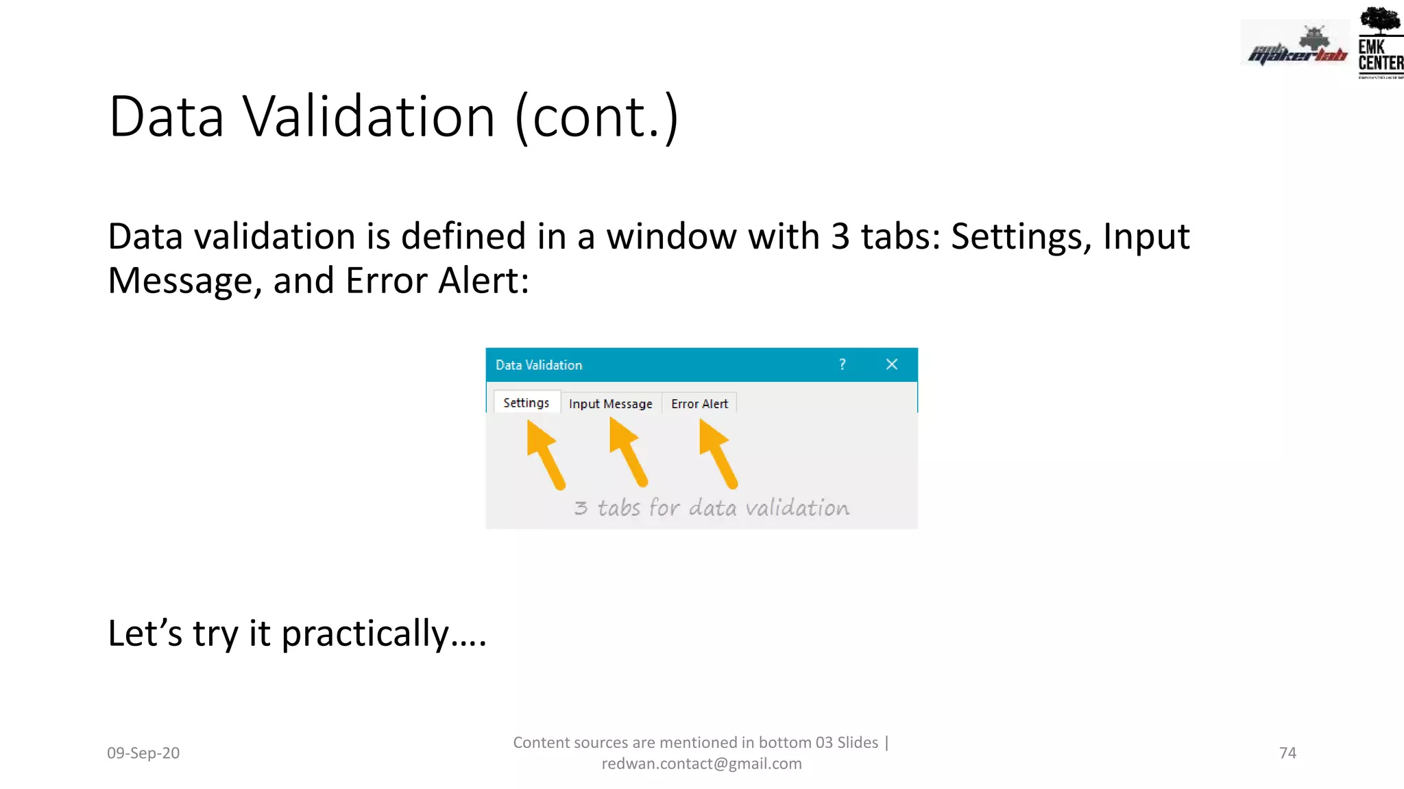
Data validation techniques to ensure data integrity and guided input in Excel spreadsheets.
Use of macros to automate repetitive tasks in Excel, improving efficiency and functionality.
Bibliography of resources and references used throughout the presentation for further learning.
Concluding the presentation with an invitation for questions and feedback from attendees.


![Road to 4th Industrial Revolution [for NDC Science Club]](https://cdn.slidesharecdn.com/ss_thumbnails/roadto4thirndc12mar22-220311194333-thumbnail.jpg?width=640&height=640&fit=bounds)


![Support, Monitoring, Continuous Improvement & Scaling Agentic Automation [3/3]](https://cdn.slidesharecdn.com/ss_thumbnails/agenticcommunityseries-day3-cfd-251120170304-ddef8112-thumbnail.jpg?width=640&height=640&fit=bounds)


