Download as PDF, PPTX


![deep learning: evolution timeline
1. Perceptron [Frank Rosenblatt, 1959]
2. Neocognitron [K Fukushima, 1980]
3. Convolutional Neural Network (CNN) [LeCun, 1989]
4. Multi-level Hierarchy Networks [Jurgen Schmidthuber, 1992]
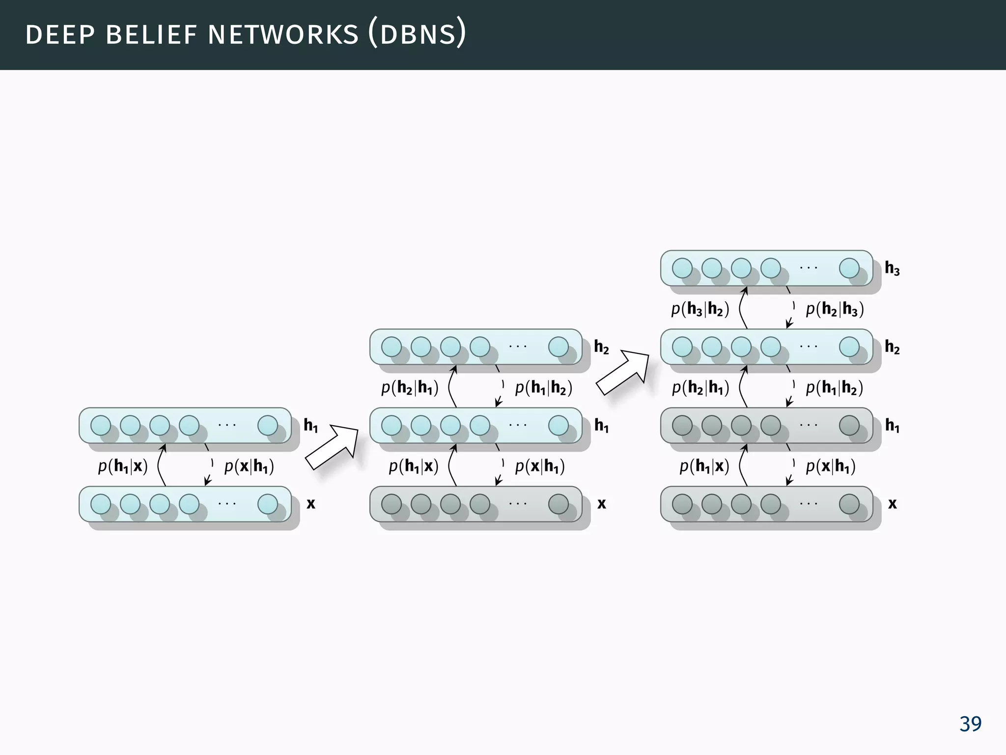
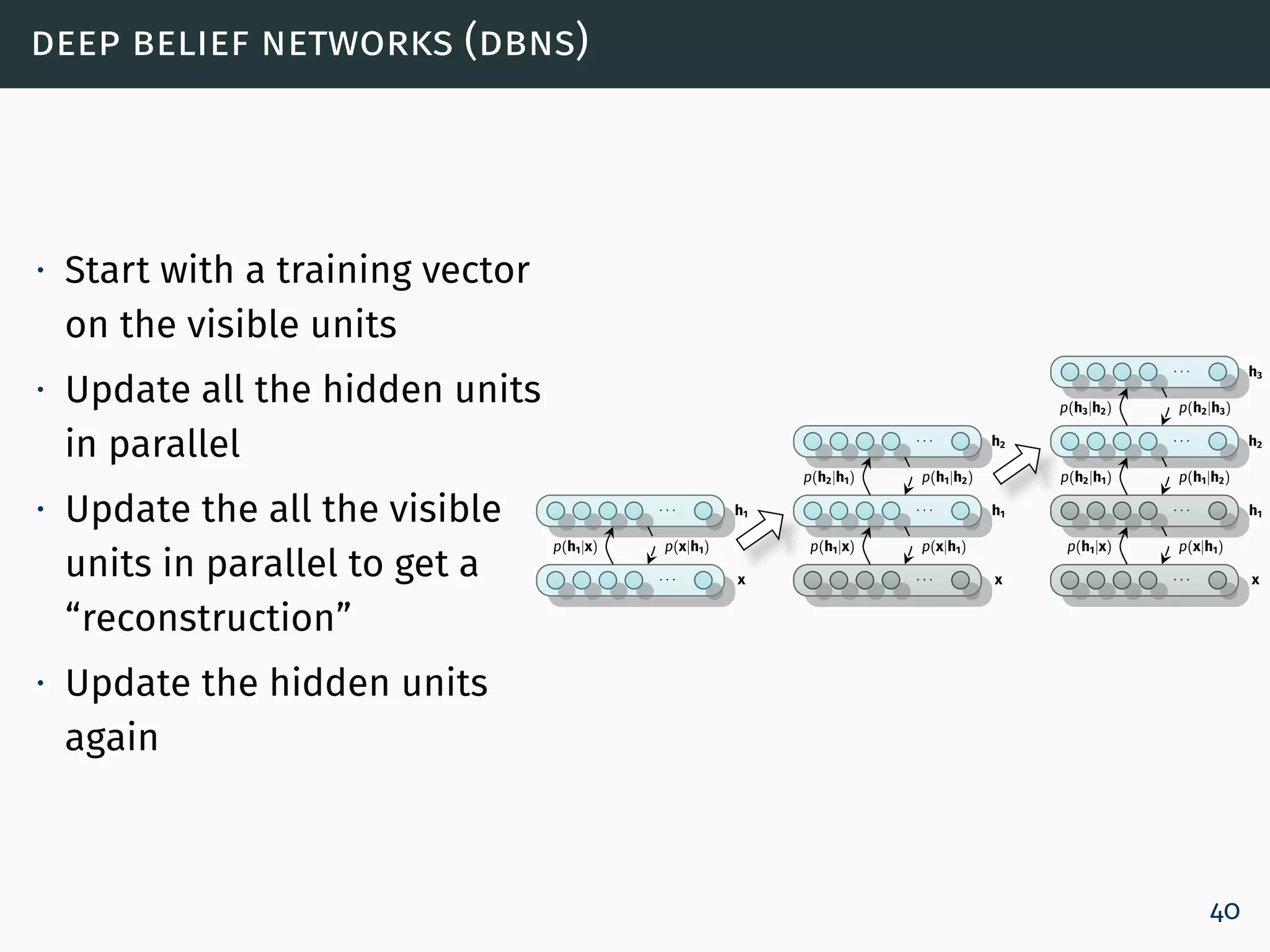
5. Deep Belief Networks (DBNs) as stack of RBMs [Geoffrey
Hinton, 2006]
6](https://image.slidesharecdn.com/dl1deeplearningalgorithms-150714090042-lva1-app6892/75/Dl1-deep-learning_algorithms-7-2048.jpg)

![from brain-like computing to deep learning
∙ New empirical and theoretical results have brought deep
architectures into the focus of the Machine Learning (ML)
researchers [Larochelle et al., 2007].
∙ Theoretical results suggest that deep architectures are
fundamental to learn the kind of brain-like complicated
functions that can represent high-level abstractions (e.g.
vision, speech, language) [Bengio, 2009]
8](https://image.slidesharecdn.com/dl1deeplearningalgorithms-150714090042-lva1-app6892/75/Dl1-deep-learning_algorithms-9-2048.jpg)

![deep neural networks
∙ Convolutional Neural Networks (CNNs) [LeCun et al., 1989]
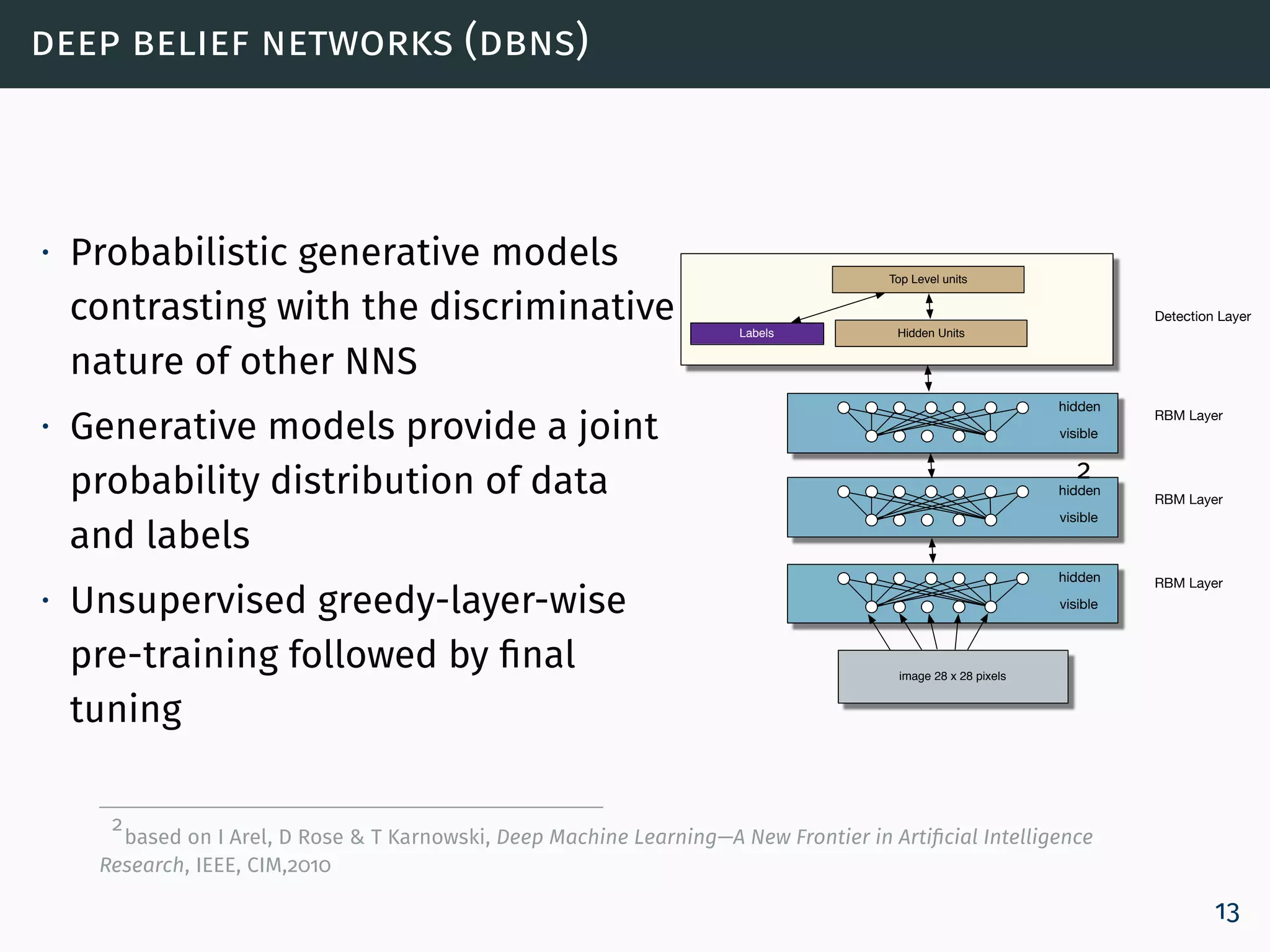
∙ Deep Belief Networks (DBNs) [Hinton et al, 2006]
∙ AutoEncoders (AEs) [Bengio et al, NIPS 2006]
∙ Sparse Autoencoders [Ranzato et al, NIPS’2006]
10](https://image.slidesharecdn.com/dl1deeplearningalgorithms-150714090042-lva1-app6892/75/Dl1-deep-learning_algorithms-11-2048.jpg)


![deep architectures versus shallow architectures
∙ Deep architectures can be exponentially more efficient
than shallow architectures [Roux and Bengio, 2010].
∙ Functions that can be compactly represented with a Neural
Network (NN) of depth d, may require an exponential number
of computational elements for a network with depth d − 1
[Bengio, 2009].
15](https://image.slidesharecdn.com/dl1deeplearningalgorithms-150714090042-lva1-app6892/75/Dl1-deep-learning_algorithms-16-2048.jpg)
![deep architectures versus shallow architectures
∙ Deep architectures can be exponentially more efficient
than shallow architectures [Roux and Bengio, 2010].
∙ Functions that can be compactly represented with a Neural
Network (NN) of depth d, may require an exponential number
of computational elements for a network with depth d − 1
[Bengio, 2009].
∙ Since the number of computational elements depends on
the number of training samples available, using shallow
architectures may result in poor generalization
models [Bengio, 2009].
∙ As a result, deep architecture models tend to outperform
shallow models such as SVMs [Larochelle et al., 2007].
15](https://image.slidesharecdn.com/dl1deeplearningalgorithms-150714090042-lva1-app6892/75/Dl1-deep-learning_algorithms-17-2048.jpg)


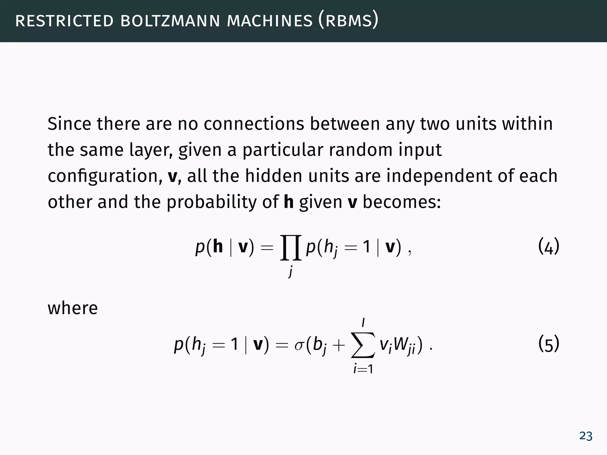
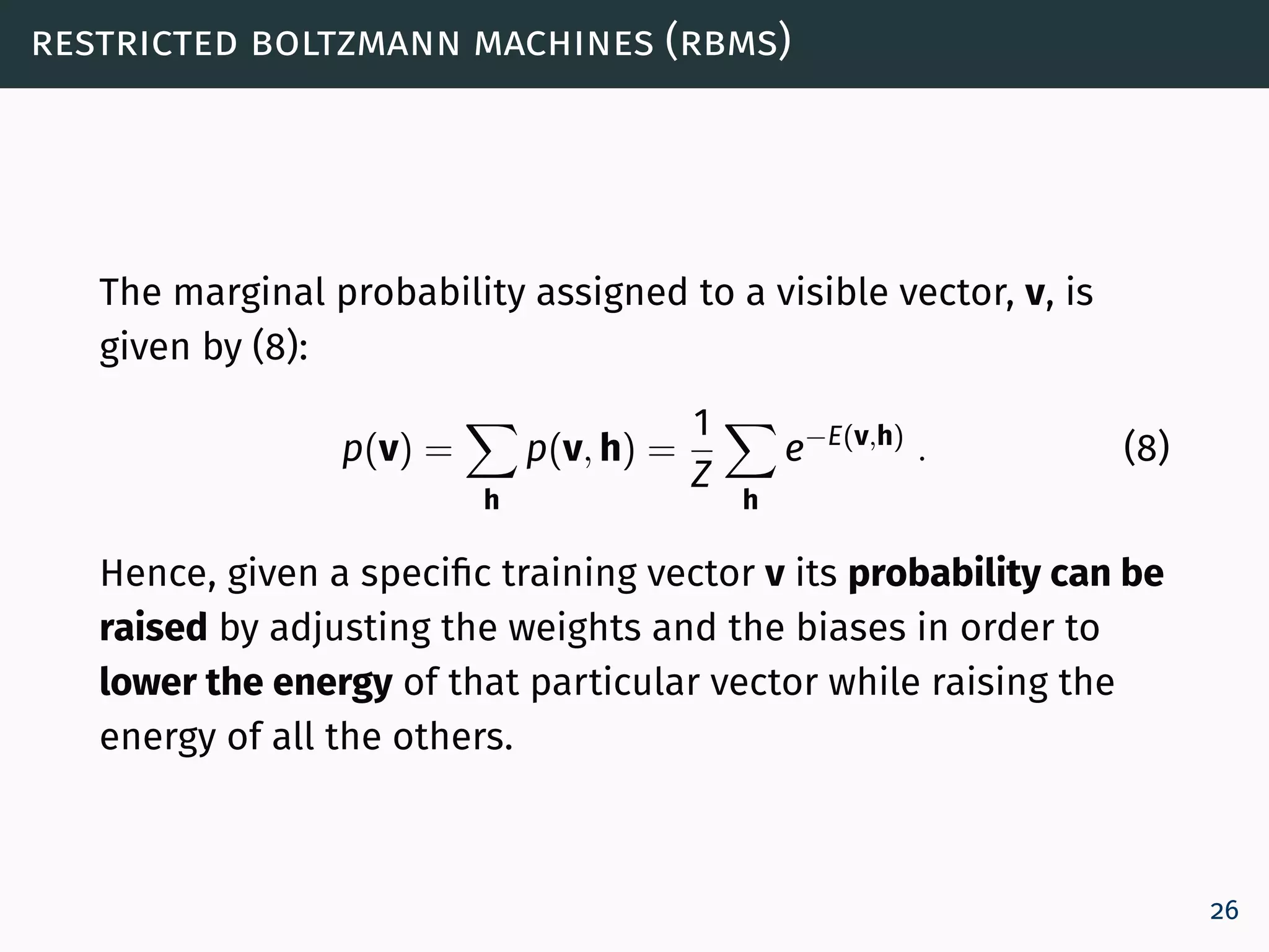
![restricted boltzmann machines (rbms)
The Restricted Boltzmann Machine (RBM) assigns a
probability for each configuration (v, h), using:
p(v, h) =
e−E(v,h)
Z
, (2)
where Z is a normalization constant called partition function,
obtained by summing up the energy of all possible (v, h)
configurations [Bengio, 2009, Hinton, 2010,
Carreira-Perpiñán and Hinton, 2005]:
Z =
v,h
e−E(v,h)
. (3)
22](https://image.slidesharecdn.com/dl1deeplearningalgorithms-150714090042-lva1-app6892/75/Dl1-deep-learning_algorithms-24-2048.jpg)


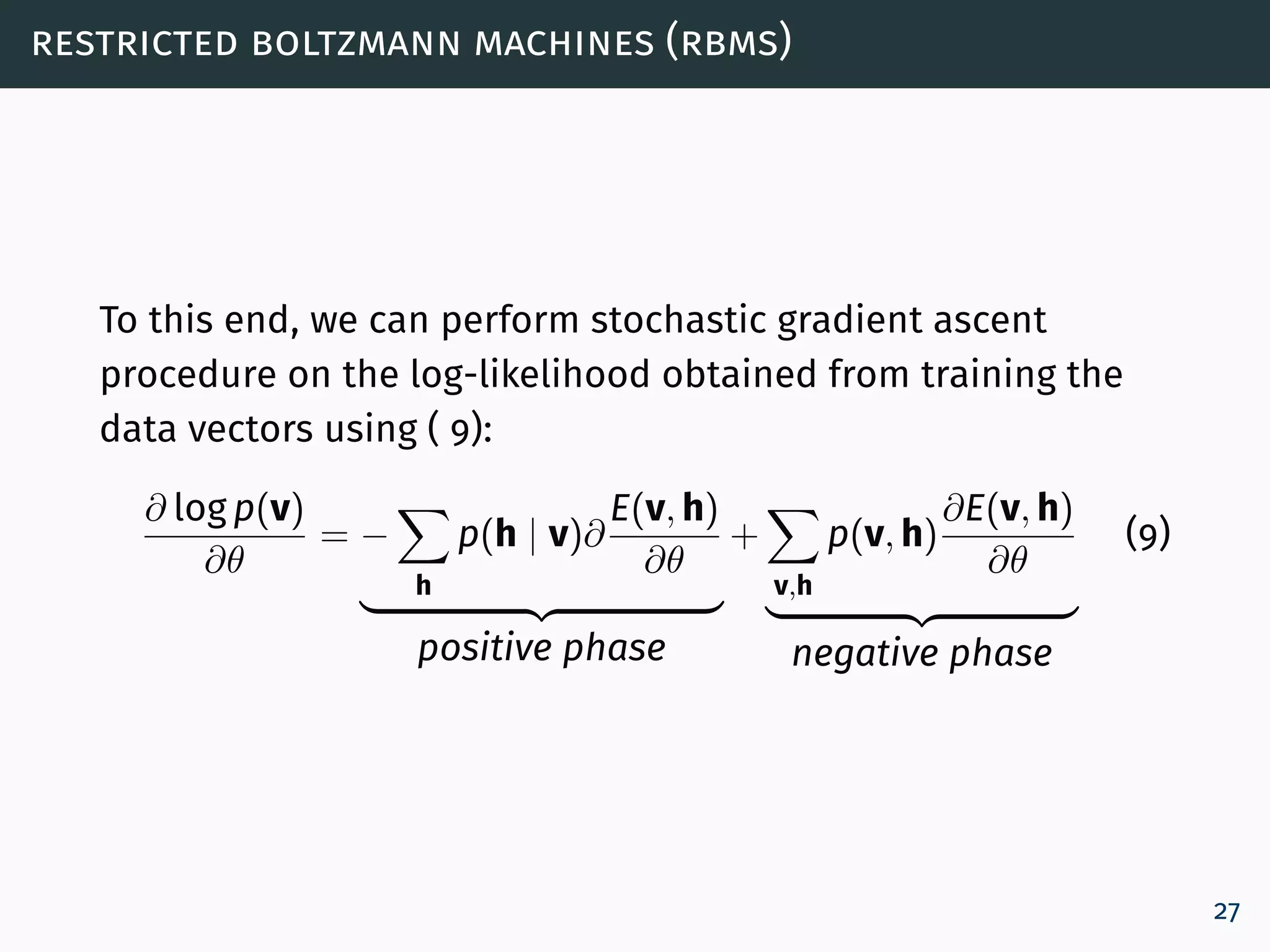

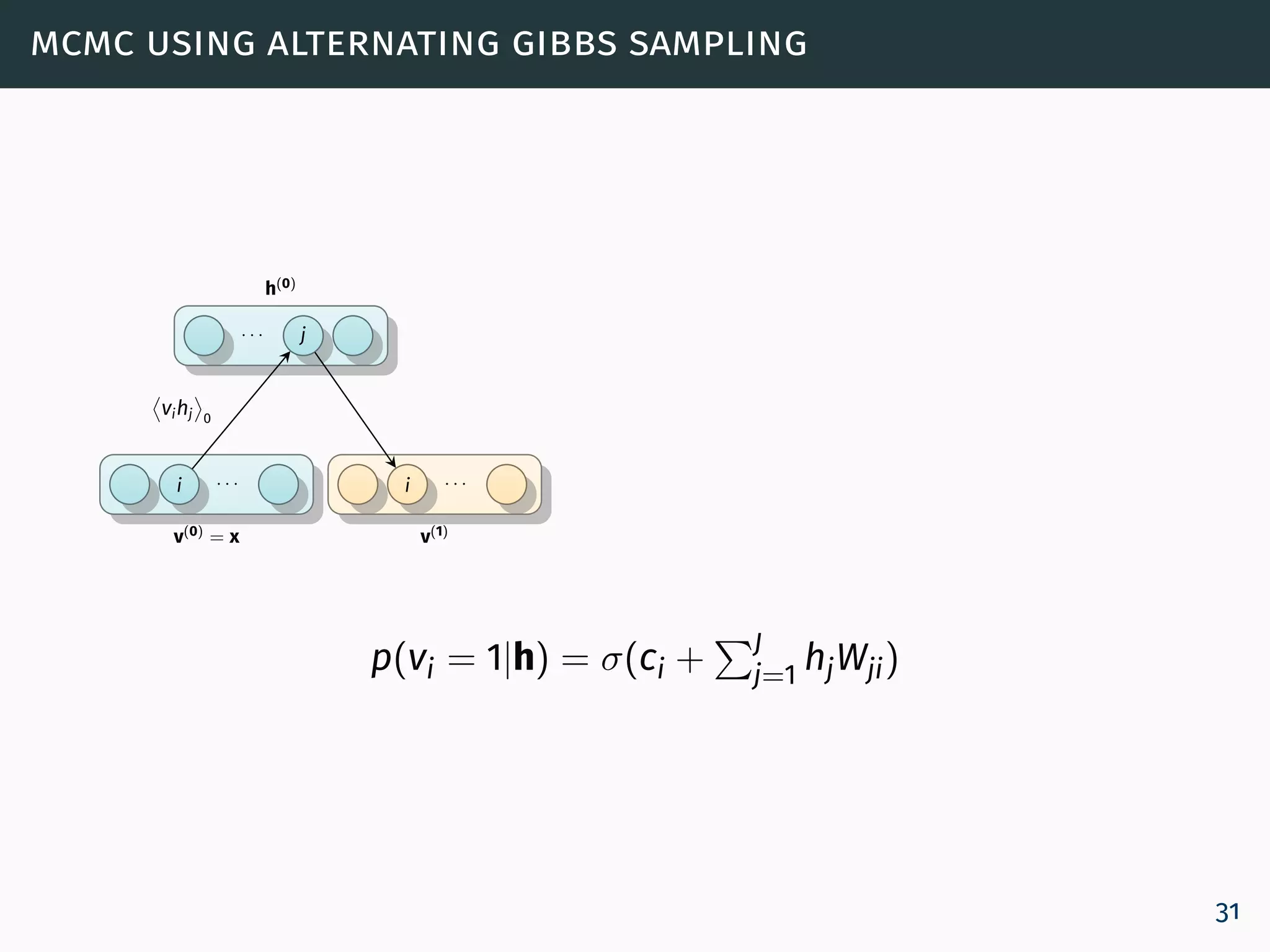
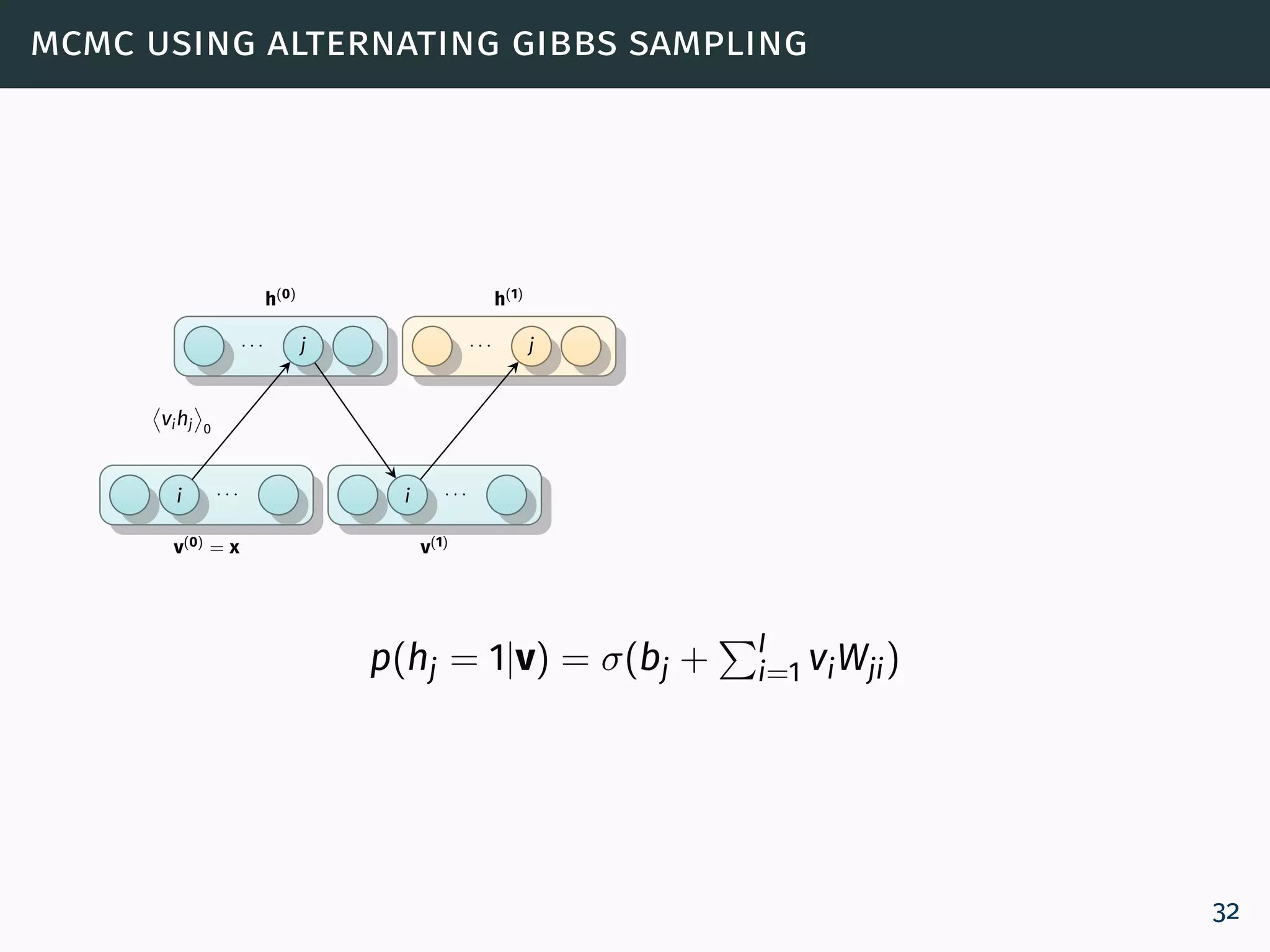
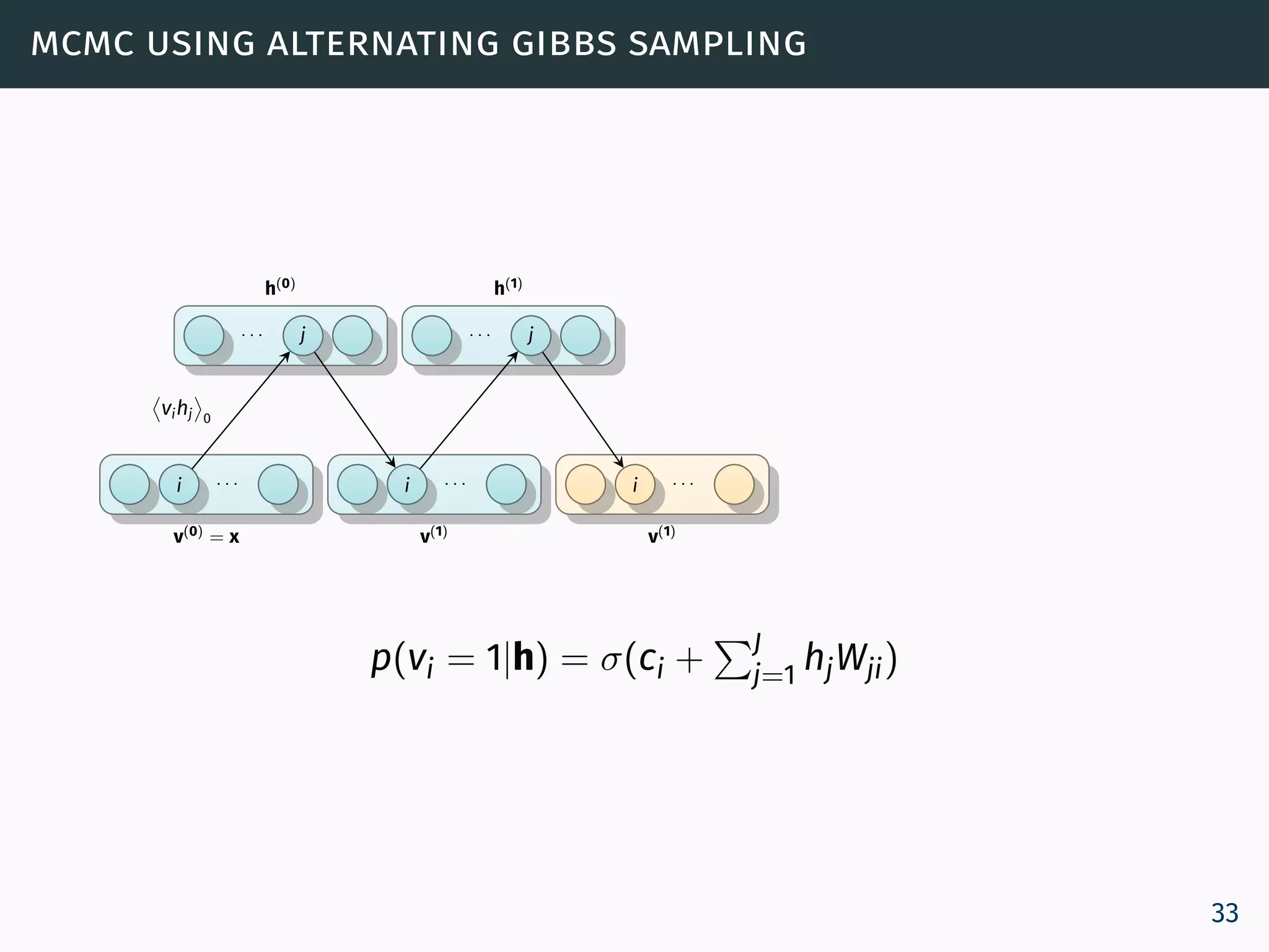
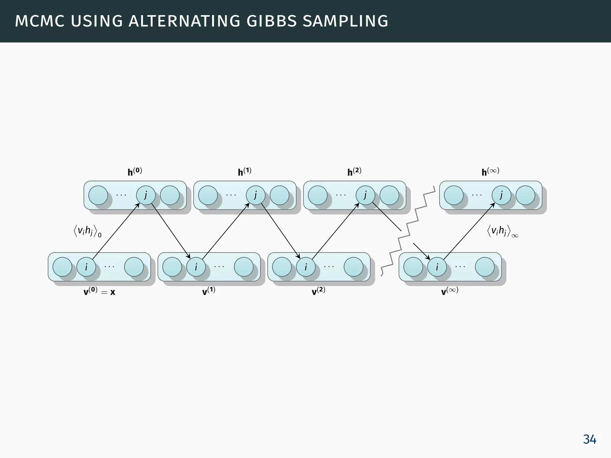
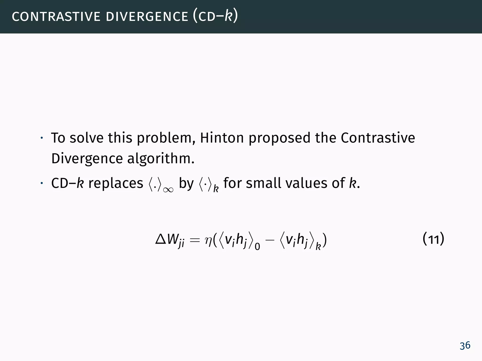
![training an rbm
The learning rule for performing stochastic steepest ascent in
the log probability of the training data:
∂ log p(v)
∂θ
= vihj 0
− vihj ∞
(10)
where · 0 denotes expectations for the data distribution
(p0 = p(h | v)) and · ∞ denotes expectations under the
model distribution
p∞(v, h) = p(v, h) [Roux and Bengio, 2008].
h1 h2 h3 · · · hj · · · hJ 1
bias
v1 v2 · · · vi · · · vI 1
bias
visible units
hidden units
decoder
encoder
29](https://image.slidesharecdn.com/dl1deeplearningalgorithms-150714090042-lva1-app6892/75/Dl1-deep-learning_algorithms-31-2048.jpg)


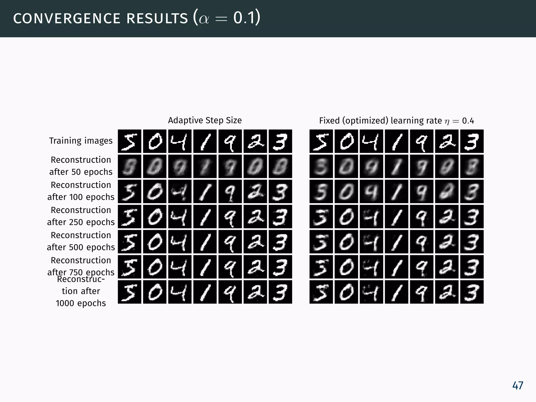
![deep belief networks (dbns) - adaptive learning rate size
ηji =
uη(old)
ji
if ( vihj 0
− vihj k
)( vihj
(old)
0
− vihj
(old)
k
) > 0
dη(old)
ji
if ( vihj 0
− vihj k
)( vihj
(old)
0
− vihj
(old)
k
) < 0
4
4
Lopes et al., Towards Adaptive learning with improved
convergence of DBNs on GPUs, Pattern Recognition, [2014]
45](https://image.slidesharecdn.com/dl1deeplearningalgorithms-150714090042-lva1-app6892/75/Dl1-deep-learning_algorithms-47-2048.jpg)


![deep learning: evolution timeline
1. Perceptron [Frank Rosenblatt, 1959]
2. Neocognitron [K Fukushima, 1980]
3. Convolutional Neural Network (CNN) [LeCun, 1989]
4. Multi-level Hierarchy Networks [Jurgen Schmidthuber, 1992]
5. Deep Belief Networks (DBNs) as stack of RBMs [Geoffrey
Hinton, 2006]
6](https://crownmelresort.com/image.slidesharecdn.com/dl1deeplearningalgorithms-150714090042-lva1-app6892/75/Dl1-deep-learning_algorithms-7-2048.jpg)

![from brain-like computing to deep learning
∙ New empirical and theoretical results have brought deep
architectures into the focus of the Machine Learning (ML)
researchers [Larochelle et al., 2007].
∙ Theoretical results suggest that deep architectures are
fundamental to learn the kind of brain-like complicated
functions that can represent high-level abstractions (e.g.
vision, speech, language) [Bengio, 2009]
8](https://crownmelresort.com/image.slidesharecdn.com/dl1deeplearningalgorithms-150714090042-lva1-app6892/75/Dl1-deep-learning_algorithms-9-2048.jpg)

![deep neural networks
∙ Convolutional Neural Networks (CNNs) [LeCun et al., 1989]
∙ Deep Belief Networks (DBNs) [Hinton et al, 2006]
∙ AutoEncoders (AEs) [Bengio et al, NIPS 2006]
∙ Sparse Autoencoders [Ranzato et al, NIPS’2006]
10](https://crownmelresort.com/image.slidesharecdn.com/dl1deeplearningalgorithms-150714090042-lva1-app6892/75/Dl1-deep-learning_algorithms-11-2048.jpg)


![deep architectures versus shallow architectures
∙ Deep architectures can be exponentially more efficient
than shallow architectures [Roux and Bengio, 2010].
∙ Functions that can be compactly represented with a Neural
Network (NN) of depth d, may require an exponential number
of computational elements for a network with depth d − 1
[Bengio, 2009].
15](https://crownmelresort.com/image.slidesharecdn.com/dl1deeplearningalgorithms-150714090042-lva1-app6892/75/Dl1-deep-learning_algorithms-16-2048.jpg)
![deep architectures versus shallow architectures
∙ Deep architectures can be exponentially more efficient
than shallow architectures [Roux and Bengio, 2010].
∙ Functions that can be compactly represented with a Neural
Network (NN) of depth d, may require an exponential number
of computational elements for a network with depth d − 1
[Bengio, 2009].
∙ Since the number of computational elements depends on
the number of training samples available, using shallow
architectures may result in poor generalization
models [Bengio, 2009].
∙ As a result, deep architecture models tend to outperform
shallow models such as SVMs [Larochelle et al., 2007].
15](https://crownmelresort.com/image.slidesharecdn.com/dl1deeplearningalgorithms-150714090042-lva1-app6892/75/Dl1-deep-learning_algorithms-17-2048.jpg)


![restricted boltzmann machines (rbms)
The Restricted Boltzmann Machine (RBM) assigns a
probability for each configuration (v, h), using:
p(v, h) =
e−E(v,h)
Z
, (2)
where Z is a normalization constant called partition function,
obtained by summing up the energy of all possible (v, h)
configurations [Bengio, 2009, Hinton, 2010,
Carreira-Perpiñán and Hinton, 2005]:
Z =
v,h
e−E(v,h)
. (3)
22](https://crownmelresort.com/image.slidesharecdn.com/dl1deeplearningalgorithms-150714090042-lva1-app6892/75/Dl1-deep-learning_algorithms-24-2048.jpg)


![training an rbm
The learning rule for performing stochastic steepest ascent in
the log probability of the training data:
∂ log p(v)
∂θ
= vihj 0
− vihj ∞
(10)
where · 0 denotes expectations for the data distribution
(p0 = p(h | v)) and · ∞ denotes expectations under the
model distribution
p∞(v, h) = p(v, h) [Roux and Bengio, 2008].
h1 h2 h3 · · · hj · · · hJ 1
bias
v1 v2 · · · vi · · · vI 1
bias
visible units
hidden units
decoder
encoder
29](https://crownmelresort.com/image.slidesharecdn.com/dl1deeplearningalgorithms-150714090042-lva1-app6892/75/Dl1-deep-learning_algorithms-31-2048.jpg)


![deep belief networks (dbns) - adaptive learning rate size
ηji =
uη(old)
ji
if ( vihj 0
− vihj k
)( vihj
(old)
0
− vihj
(old)
k
) > 0
dη(old)
ji
if ( vihj 0
− vihj k
)( vihj
(old)
0
− vihj
(old)
k
) < 0
4
4
Lopes et al., Towards Adaptive learning with improved
convergence of DBNs on GPUs, Pattern Recognition, [2014]
45](https://crownmelresort.com/image.slidesharecdn.com/dl1deeplearningalgorithms-150714090042-lva1-app6892/75/Dl1-deep-learning_algorithms-47-2048.jpg)


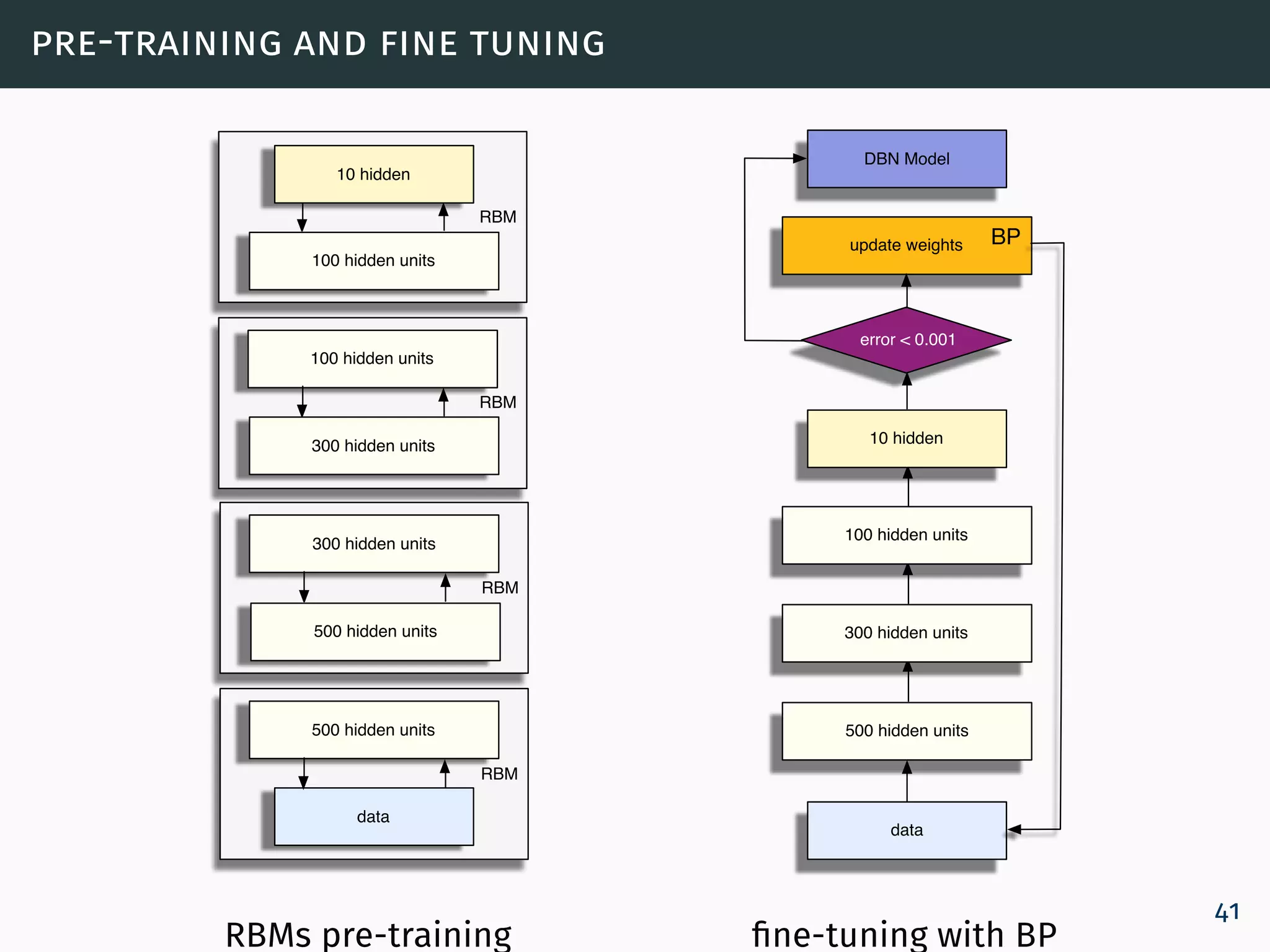
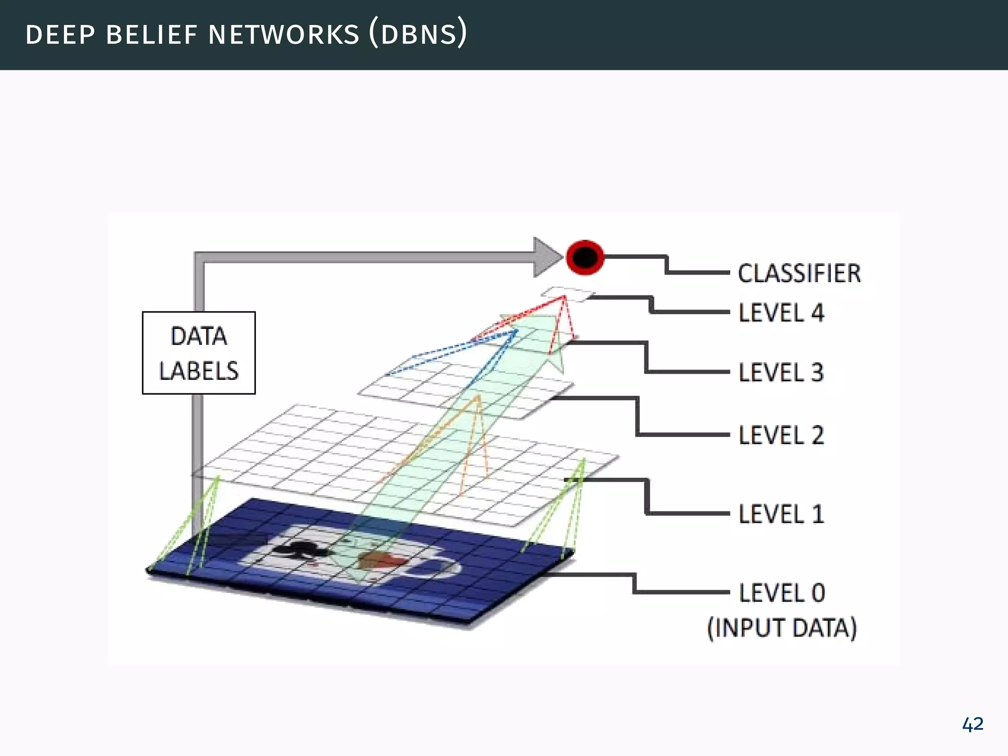
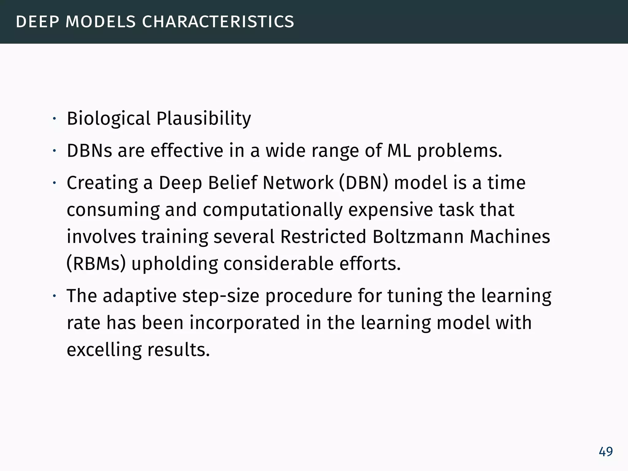
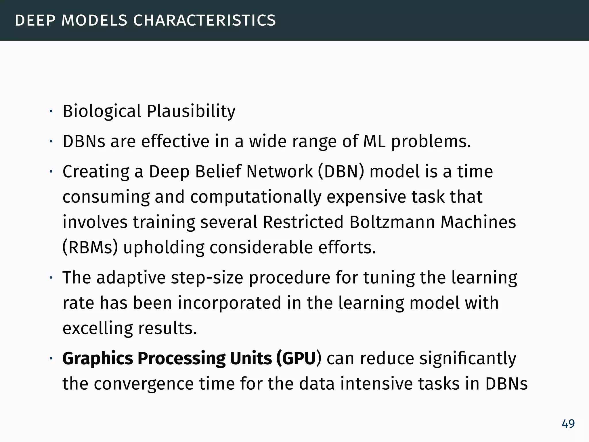
This document provides an overview of deep learning algorithms, including deep neural networks, convolutional neural networks, deep belief networks, and restricted Boltzmann machines. It discusses key concepts such as learning in deep neural networks, the evolution timeline of deep learning approaches, deep architectures, and restricted Boltzmann machines. It also covers training restricted Boltzmann machines using contrastive divergence, constructing deep belief networks by stacking restricted Boltzmann machines, and practical considerations for pre-training and fine-tuning deep belief networks.

![[Paper] learning video representations from correspondence proposals](https://cdn.slidesharecdn.com/ss_thumbnails/paperlearningvideorepresentationsfromcorrespondenceproposals-210410235049-thumbnail.jpg?width=640&height=640&fit=bounds)


![[DSC 2016] 系列活動:李宏毅 / 一天搞懂深度學習](https://cdn.slidesharecdn.com/ss_thumbnails/1-160521014039-thumbnail.jpg?width=640&height=640&fit=bounds)