Downloaded 195 times


![Machine Learning - Dimensionality Reduction
PCA- Principal Components - SVD
SVD can implemented in scikit-learn using the code below
● SVD assumes that the data is centered around the origin
# Data needs to centralized before performing SVD
>>> X_centered = X - X.mean(axis=0)
# Performing SVD
>>> U,s,V = np.linalg.svd(X_centered)
# Printing the principal components
>>> c1, c2 = V.T[:,0], V.T[:,1]
print(c1,c2)
Q. How many principal components are we printing in the above code?](https://image.slidesharecdn.com/8-180514114339/75/Dimensionality-Reduction-Machine-Learning-CloudxLab-53-2048.jpg)
![Machine Learning - Dimensionality Reduction
PCA- Principal Components - SVD
SVD can implemented in scikit-learn using the code below
● SVD assumes that the data is centered around the origin
# Data needs to centralized before performing SVD
>>> X_centered = X - X.mean(axis=0)
# Performing SVD
>>> U,s,V = np.linalg.svd(X_centered)
# Printing the principal components
>>> c1, c2 = V.T[:,0], V.T[:,1]
print(c1,c2)
Q. How many principal components are we printing in the above code?
Ans: 2](https://image.slidesharecdn.com/8-180514114339/75/Dimensionality-Reduction-Machine-Learning-CloudxLab-54-2048.jpg)
![Machine Learning - Dimensionality Reduction
PCA- SVD and PCA
PCA using SVD in Sci-kit Learn PCA using Sci-kit Learn PCA function
# Centering the data and doing SVD
X_centered = X - X.mean(axis=0)
U,s,V = np.linalg.svd(X_centered)
# Extracting the components and projecting the
# original dataset
W2 = V.T[:, :2]
X2D = X_centered.dot(W2)
from sklearn.decomposition import PCA
# Directly doing PCA and transforming the
original dataset
# Takes care of centering
pca = PCA(n_components = 2)
X2D = pca.fit_transform(X)
Switch to Notebook](https://image.slidesharecdn.com/8-180514114339/75/Dimensionality-Reduction-Machine-Learning-CloudxLab-59-2048.jpg)
![Machine Learning - Dimensionality Reduction
PCA- Explained Variance Ratio
Variances explained by each of the components is important
● We would like to cover as much variance as in the original dataset
● available via the explained_variance_ratio_ variable
>>> print(pca.explained_variance_ratio_)
[ 0.95369864 0.04630136]
1st component
covers 95.3 % of
the variance
2nd component
covers 4.6 % of
the variance](https://image.slidesharecdn.com/8-180514114339/75/Dimensionality-Reduction-Machine-Learning-CloudxLab-60-2048.jpg)
![Machine Learning - Dimensionality Reduction
PCA- Compression of dataset - Demo
Loading the MNIST Dataset
#MNIST compression:
>>> from sklearn.model_selection import train_test_split
>>> from sklearn.datasets import fetch_mldata
>>> mnist = fetch_mldata('MNIST original')
>>> X, y = mnist["data"], mnist["target"]
>>> X_train, X_test, y_train, y_test = train_test_split(X, y)
>>> X = X_train](https://image.slidesharecdn.com/8-180514114339/75/Dimensionality-Reduction-Machine-Learning-CloudxLab-67-2048.jpg)
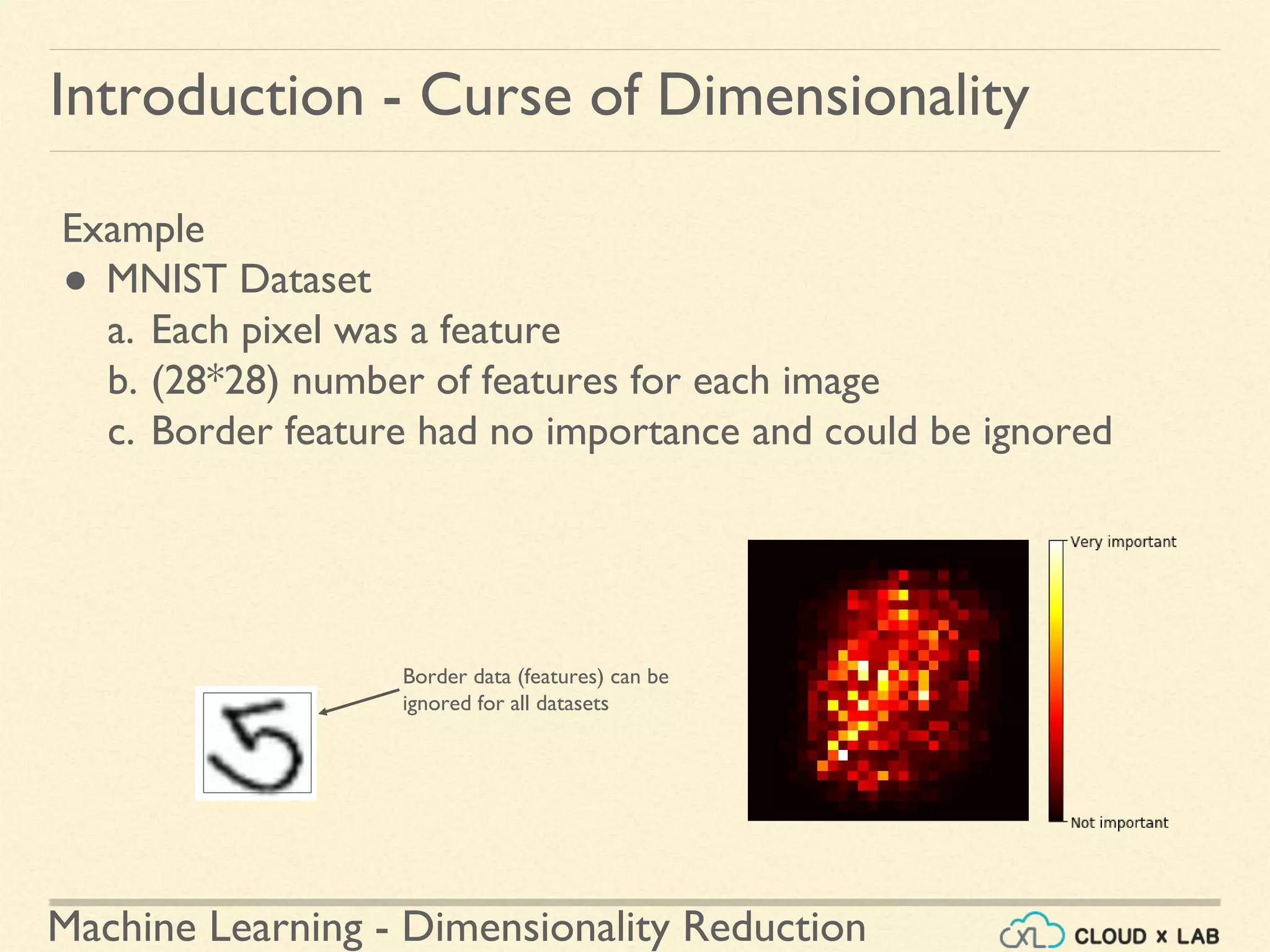
![Machine Learning - Dimensionality Reduction
PCA- Incremental PCA
Another way is to use Numpy memap class
● Uses binary array on the disk as if it was in-memory
# alternative: Numpy memmap class (use binary array on disk as if it was in memory)
>>> filename = "my_mnist.data"
>>> X_mm = np.memmap(
filename, dtype='float32', mode='write', shape=X_mnist.shape)
>>> X_mm[:] = X_mnist
>>> del X_mm
>>> X_mm = np.memmap(filename, dtype='float32', mode='readonly', shape=X_mnist.shape)
>>> batch_size = len(X_mnist) // n_batches
>>> inc_pca = IncrementalPCA(n_components=154, batch_size=batch_size)
>>> inc_pca.fit(X_mm)
Switch to Notebook](https://image.slidesharecdn.com/8-180514114339/75/Dimensionality-Reduction-Machine-Learning-CloudxLab-73-2048.jpg)
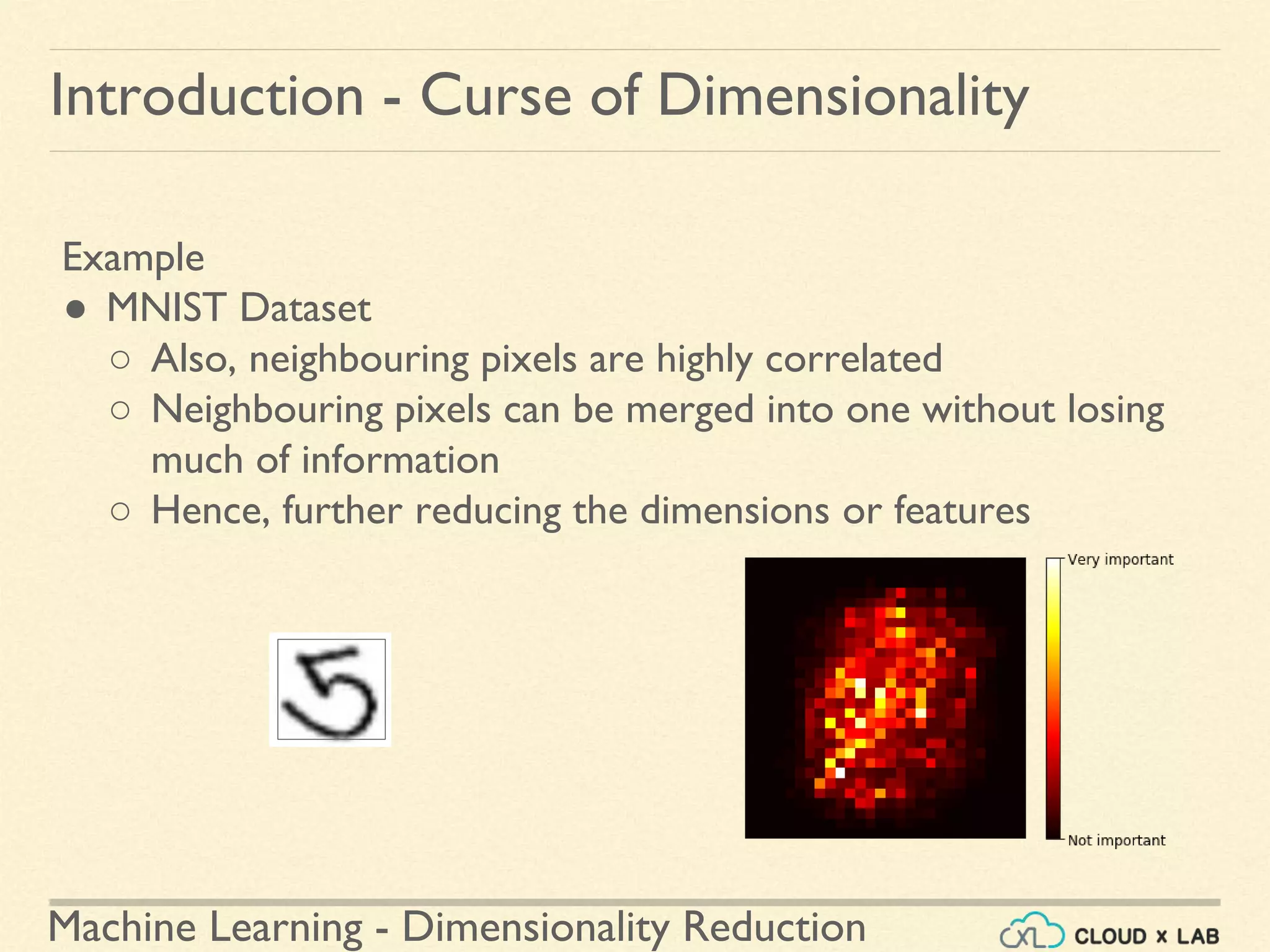
![Machine Learning - Dimensionality Reduction
Kernel PCA - Selecting hyperparameters
Selecting hyper parameters
● Create a pipeline with KernelPCA and Classification model
● Doing a grid search using GridSearchCV to find the best kernel and
gamma value for kPCA
>>> clf = Pipeline([
("kpca", KernelPCA(n_components=2)),
("log_reg", LogisticRegression())])
>>> param_grid = [{
"kpca__gamma": np.linspace(0.03, 0.05, 10),
"kpca__kernel": ["rbf", "sigmoid"]}]
>>> grid_search = GridSearchCV(clf, param_grid, cv=3)
Switch to Notebook](https://image.slidesharecdn.com/8-180514114339/75/Dimensionality-Reduction-Machine-Learning-CloudxLab-79-2048.jpg)
![Machine Learning - Dimensionality Reduction
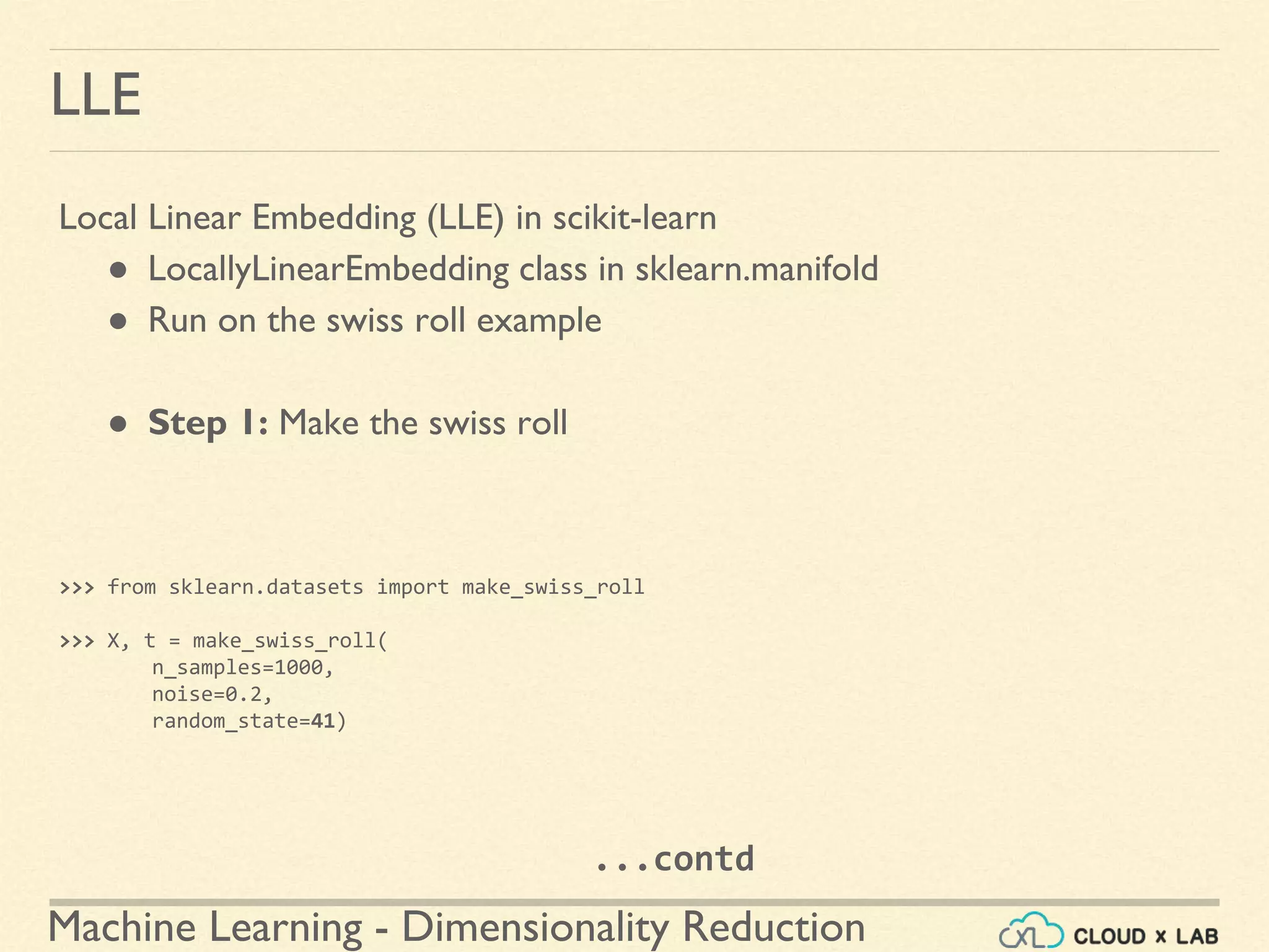
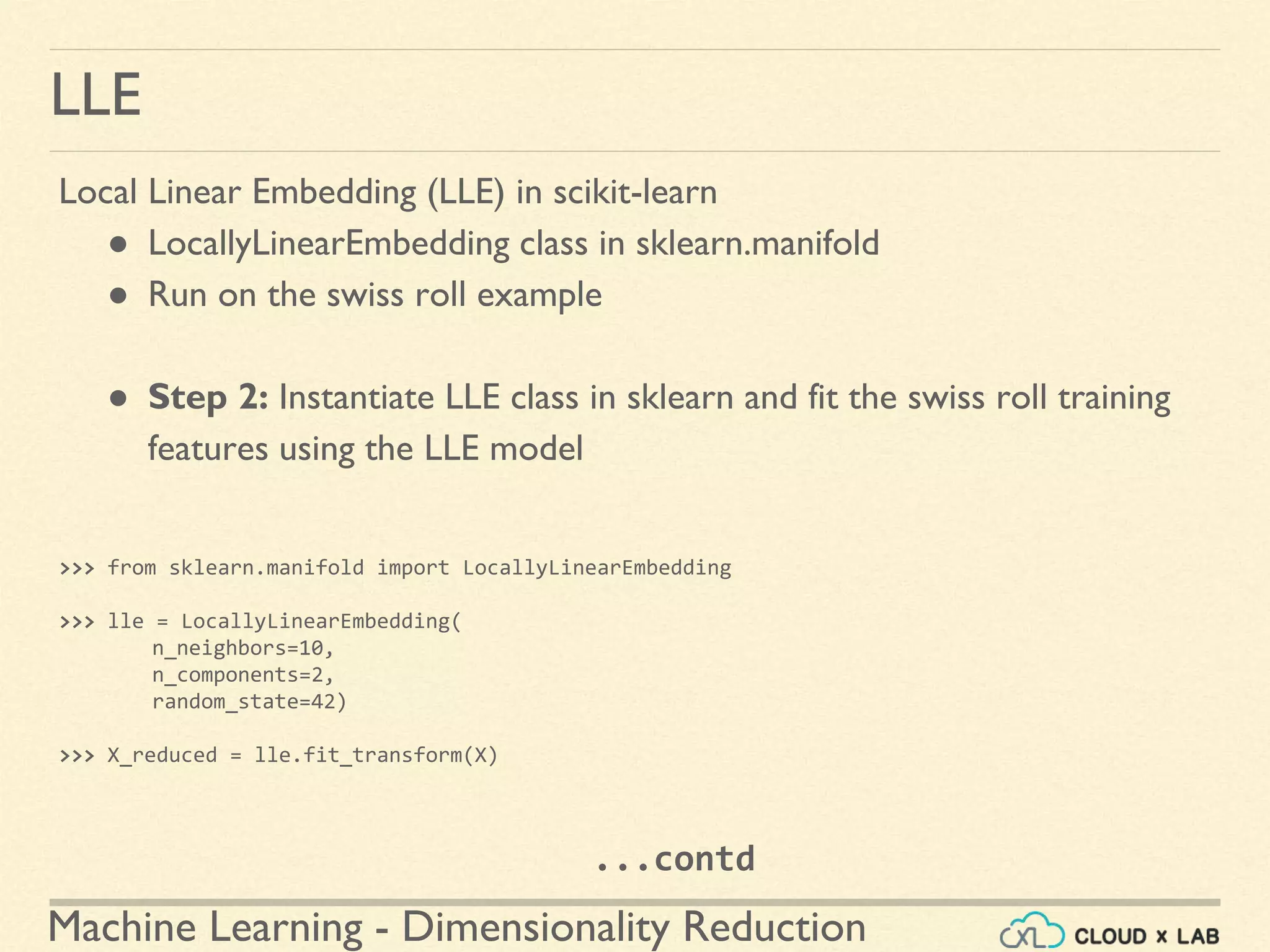
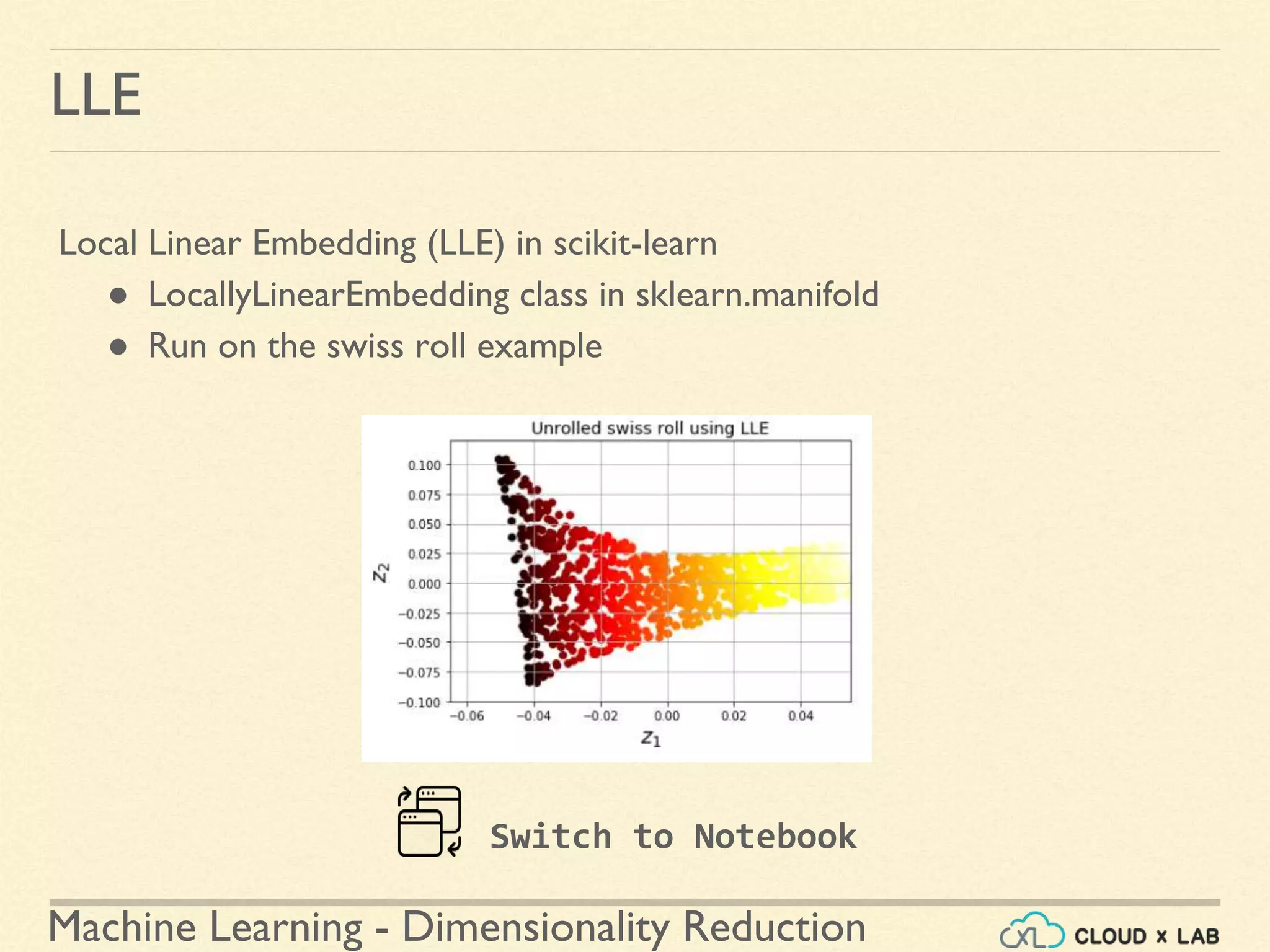
LLE
Local Linear Embedding (LLE) in scikit-learn
● LocallyLinearEmbedding class in sklearn.manifold
● Run on the swiss roll example
● Step 3: Plot the reduced dimension data
>>> plt.title("Unrolled swiss roll using LLE", fontsize=14)
>>> plt.scatter(X_reduced[:, 0], X_reduced[:, 1], c=t, cmap=plt.cm.hot)
>>> plt.xlabel("$z_1$", fontsize=18)
>>> plt.ylabel("$z_2$", fontsize=18)
>>> plt.axis([-0.065, 0.055, -0.1, 0.12])
>>> plt.grid(True)
>>> plt.show()
...contd](https://image.slidesharecdn.com/8-180514114339/75/Dimensionality-Reduction-Machine-Learning-CloudxLab-90-2048.jpg)
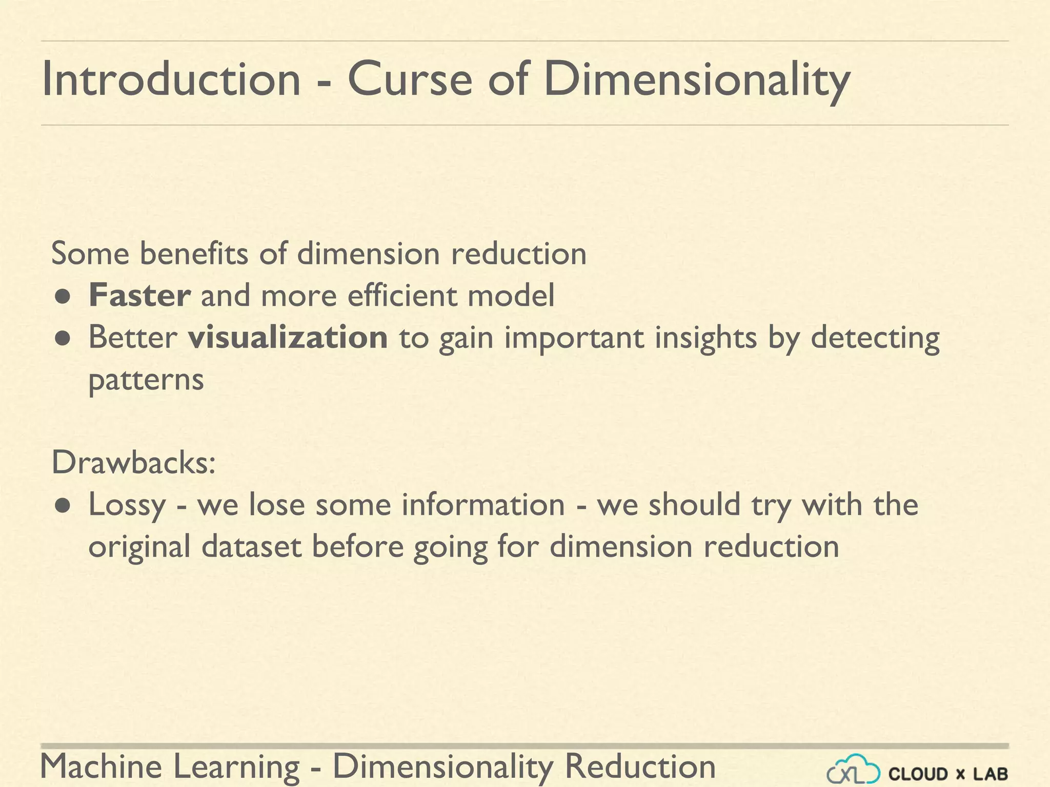
![Machine Learning - Dimensionality Reduction
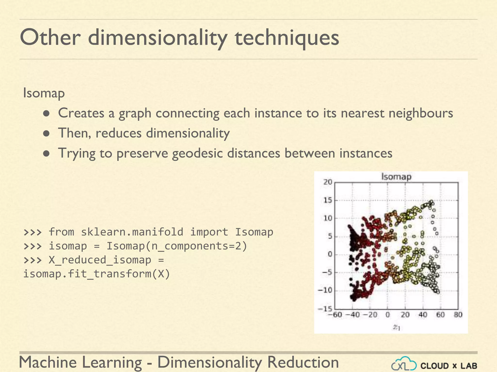
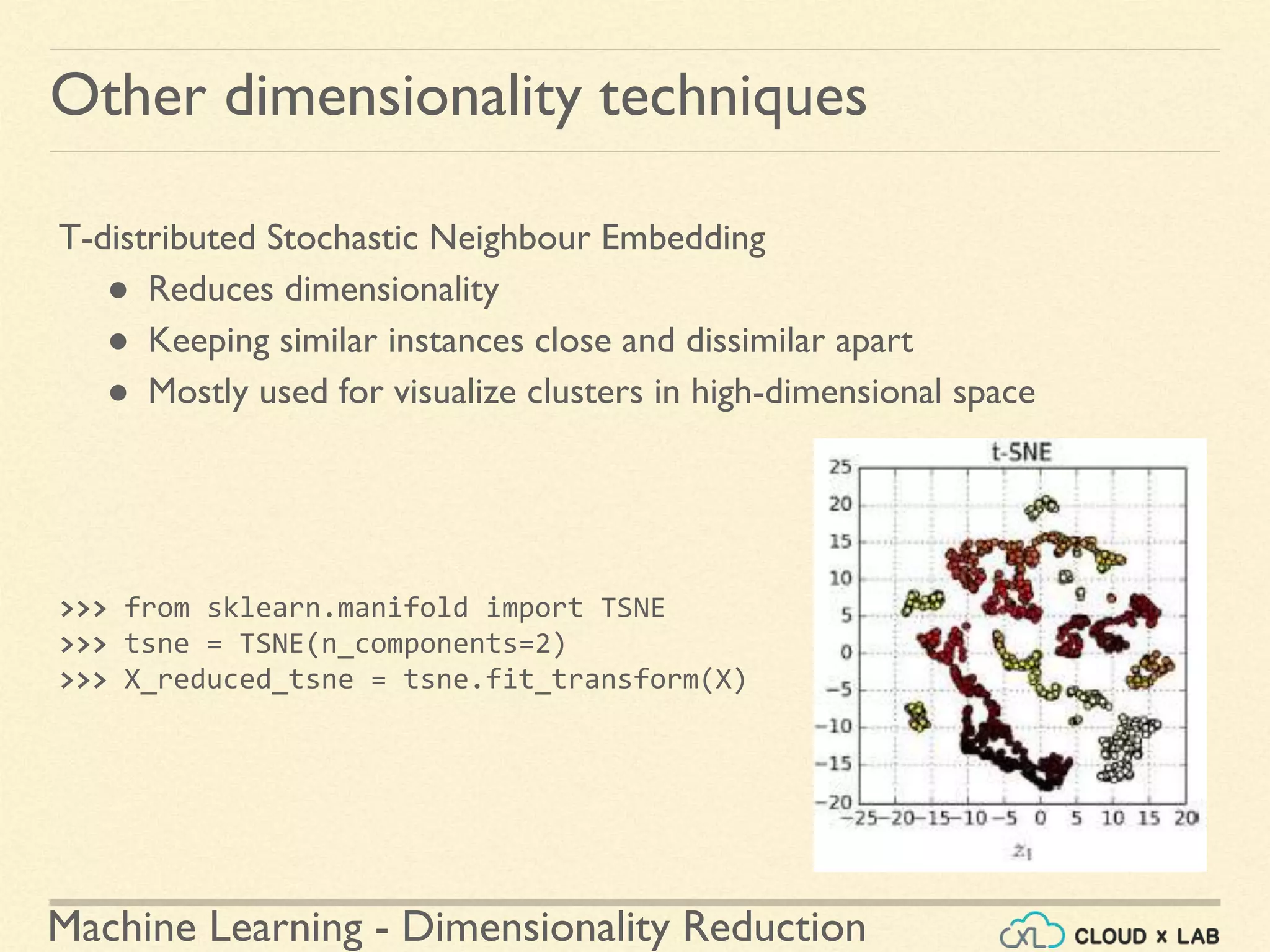
Other dimensionality techniques
Plotting the results for each of the techniques on the notebook
>>> titles = ["MDS", "Isomap", "t-SNE"]
>>> plt.figure(figsize=(11,4))
for subplot, title, X_reduced in zip((131, 132, 133), titles,
(X_reduced_mds, X_reduced_isomap, X_reduced_tsne)):
plt.subplot(subplot)
plt.title(title, fontsize=14)
plt.scatter(X_reduced[:, 0], X_reduced[:, 1], c=t, cmap=plt.cm.hot)
plt.xlabel("$z_1$", fontsize=18)
if subplot == 131:
plt.ylabel("$z_2$", fontsize=18, rotation=0)
plt.grid(True)
>>> plt.show()
Switch to Notebook](https://image.slidesharecdn.com/8-180514114339/75/Dimensionality-Reduction-Machine-Learning-CloudxLab-100-2048.jpg)


![Machine Learning - Dimensionality Reduction
PCA- Principal Components - SVD
SVD can implemented in scikit-learn using the code below
● SVD assumes that the data is centered around the origin
# Data needs to centralized before performing SVD
>>> X_centered = X - X.mean(axis=0)
# Performing SVD
>>> U,s,V = np.linalg.svd(X_centered)
# Printing the principal components
>>> c1, c2 = V.T[:,0], V.T[:,1]
print(c1,c2)
Q. How many principal components are we printing in the above code?](https://crownmelresort.com/image.slidesharecdn.com/8-180514114339/75/Dimensionality-Reduction-Machine-Learning-CloudxLab-53-2048.jpg)
![Machine Learning - Dimensionality Reduction
PCA- Principal Components - SVD
SVD can implemented in scikit-learn using the code below
● SVD assumes that the data is centered around the origin
# Data needs to centralized before performing SVD
>>> X_centered = X - X.mean(axis=0)
# Performing SVD
>>> U,s,V = np.linalg.svd(X_centered)
# Printing the principal components
>>> c1, c2 = V.T[:,0], V.T[:,1]
print(c1,c2)
Q. How many principal components are we printing in the above code?
Ans: 2](https://crownmelresort.com/image.slidesharecdn.com/8-180514114339/75/Dimensionality-Reduction-Machine-Learning-CloudxLab-54-2048.jpg)


![Machine Learning - Dimensionality Reduction
PCA- SVD and PCA
PCA using SVD in Sci-kit Learn PCA using Sci-kit Learn PCA function
# Centering the data and doing SVD
X_centered = X - X.mean(axis=0)
U,s,V = np.linalg.svd(X_centered)
# Extracting the components and projecting the
# original dataset
W2 = V.T[:, :2]
X2D = X_centered.dot(W2)
from sklearn.decomposition import PCA
# Directly doing PCA and transforming the
original dataset
# Takes care of centering
pca = PCA(n_components = 2)
X2D = pca.fit_transform(X)
Switch to Notebook](https://crownmelresort.com/image.slidesharecdn.com/8-180514114339/75/Dimensionality-Reduction-Machine-Learning-CloudxLab-59-2048.jpg)
![Machine Learning - Dimensionality Reduction
PCA- Explained Variance Ratio
Variances explained by each of the components is important
● We would like to cover as much variance as in the original dataset
● available via the explained_variance_ratio_ variable
>>> print(pca.explained_variance_ratio_)
[ 0.95369864 0.04630136]
1st component
covers 95.3 % of
the variance
2nd component
covers 4.6 % of
the variance](https://crownmelresort.com/image.slidesharecdn.com/8-180514114339/75/Dimensionality-Reduction-Machine-Learning-CloudxLab-60-2048.jpg)


![Machine Learning - Dimensionality Reduction
PCA- Compression of dataset - Demo
Loading the MNIST Dataset
#MNIST compression:
>>> from sklearn.model_selection import train_test_split
>>> from sklearn.datasets import fetch_mldata
>>> mnist = fetch_mldata('MNIST original')
>>> X, y = mnist["data"], mnist["target"]
>>> X_train, X_test, y_train, y_test = train_test_split(X, y)
>>> X = X_train](https://crownmelresort.com/image.slidesharecdn.com/8-180514114339/75/Dimensionality-Reduction-Machine-Learning-CloudxLab-67-2048.jpg)


![Machine Learning - Dimensionality Reduction
PCA- Incremental PCA
Another way is to use Numpy memap class
● Uses binary array on the disk as if it was in-memory
# alternative: Numpy memmap class (use binary array on disk as if it was in memory)
>>> filename = "my_mnist.data"
>>> X_mm = np.memmap(
filename, dtype='float32', mode='write', shape=X_mnist.shape)
>>> X_mm[:] = X_mnist
>>> del X_mm
>>> X_mm = np.memmap(filename, dtype='float32', mode='readonly', shape=X_mnist.shape)
>>> batch_size = len(X_mnist) // n_batches
>>> inc_pca = IncrementalPCA(n_components=154, batch_size=batch_size)
>>> inc_pca.fit(X_mm)
Switch to Notebook](https://crownmelresort.com/image.slidesharecdn.com/8-180514114339/75/Dimensionality-Reduction-Machine-Learning-CloudxLab-73-2048.jpg)


![Machine Learning - Dimensionality Reduction
Kernel PCA - Selecting hyperparameters
Selecting hyper parameters
● Create a pipeline with KernelPCA and Classification model
● Doing a grid search using GridSearchCV to find the best kernel and
gamma value for kPCA
>>> clf = Pipeline([
("kpca", KernelPCA(n_components=2)),
("log_reg", LogisticRegression())])
>>> param_grid = [{
"kpca__gamma": np.linspace(0.03, 0.05, 10),
"kpca__kernel": ["rbf", "sigmoid"]}]
>>> grid_search = GridSearchCV(clf, param_grid, cv=3)
Switch to Notebook](https://crownmelresort.com/image.slidesharecdn.com/8-180514114339/75/Dimensionality-Reduction-Machine-Learning-CloudxLab-79-2048.jpg)


![Machine Learning - Dimensionality Reduction
LLE
Local Linear Embedding (LLE) in scikit-learn
● LocallyLinearEmbedding class in sklearn.manifold
● Run on the swiss roll example
● Step 3: Plot the reduced dimension data
>>> plt.title("Unrolled swiss roll using LLE", fontsize=14)
>>> plt.scatter(X_reduced[:, 0], X_reduced[:, 1], c=t, cmap=plt.cm.hot)
>>> plt.xlabel("$z_1$", fontsize=18)
>>> plt.ylabel("$z_2$", fontsize=18)
>>> plt.axis([-0.065, 0.055, -0.1, 0.12])
>>> plt.grid(True)
>>> plt.show()
...contd](https://crownmelresort.com/image.slidesharecdn.com/8-180514114339/75/Dimensionality-Reduction-Machine-Learning-CloudxLab-90-2048.jpg)


![Machine Learning - Dimensionality Reduction
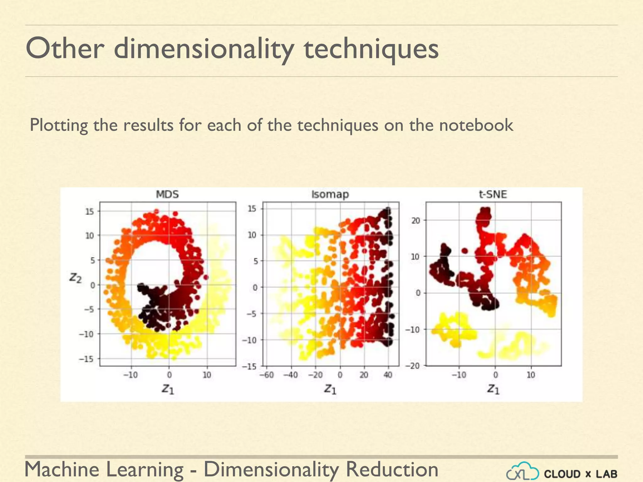
Other dimensionality techniques
Plotting the results for each of the techniques on the notebook
>>> titles = ["MDS", "Isomap", "t-SNE"]
>>> plt.figure(figsize=(11,4))
for subplot, title, X_reduced in zip((131, 132, 133), titles,
(X_reduced_mds, X_reduced_isomap, X_reduced_tsne)):
plt.subplot(subplot)
plt.title(title, fontsize=14)
plt.scatter(X_reduced[:, 0], X_reduced[:, 1], c=t, cmap=plt.cm.hot)
plt.xlabel("$z_1$", fontsize=18)
if subplot == 131:
plt.ylabel("$z_2$", fontsize=18, rotation=0)
plt.grid(True)
>>> plt.show()
Switch to Notebook](https://crownmelresort.com/image.slidesharecdn.com/8-180514114339/75/Dimensionality-Reduction-Machine-Learning-CloudxLab-100-2048.jpg)


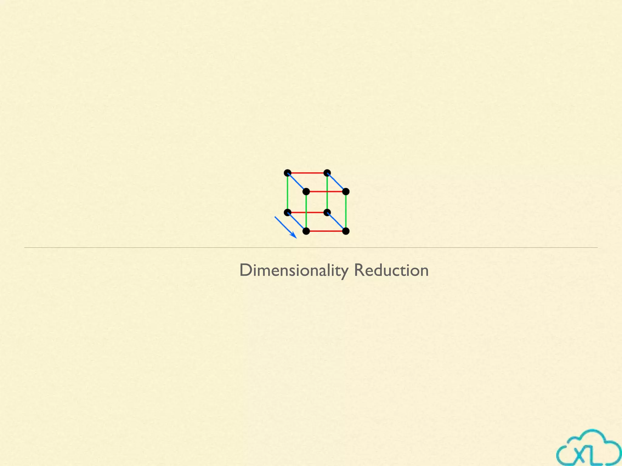
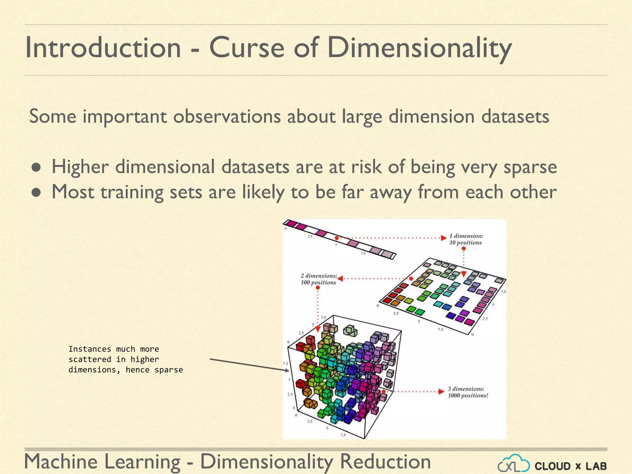
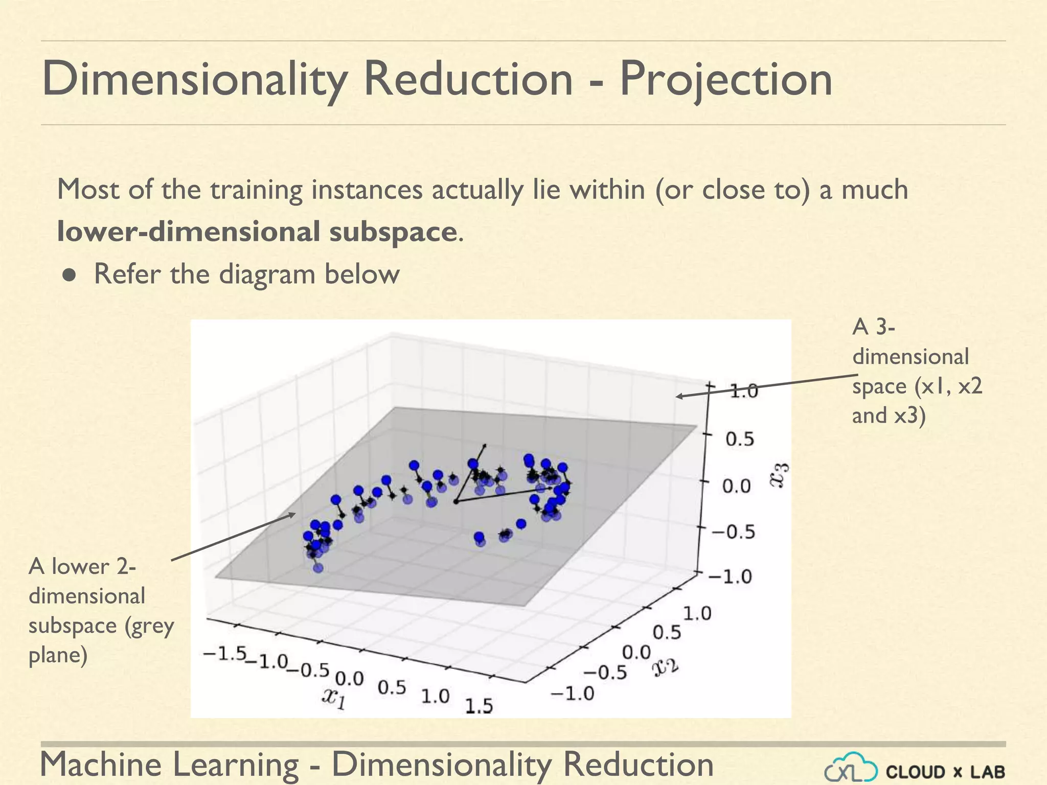
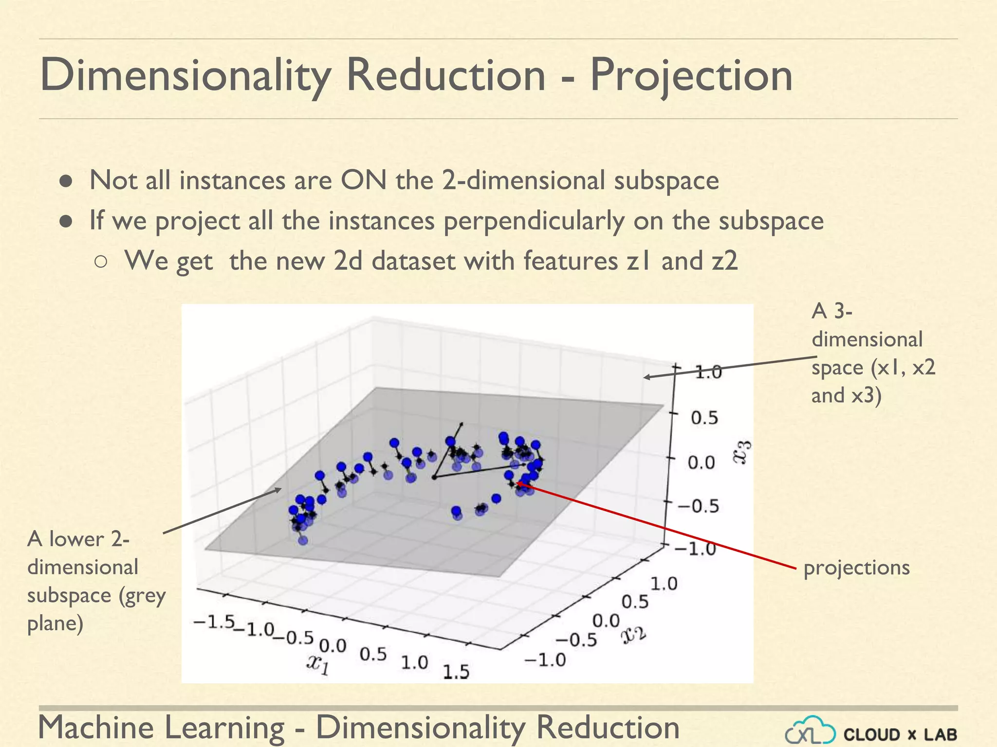
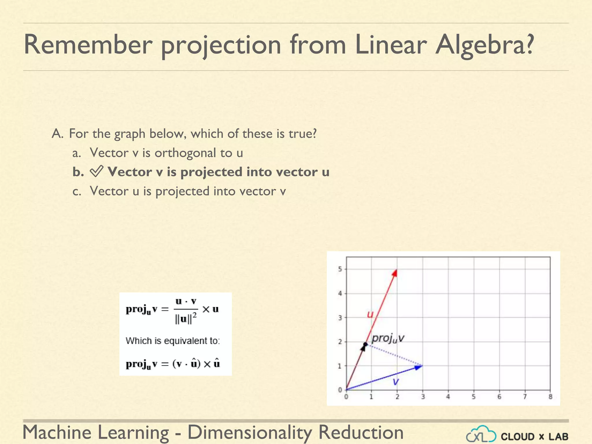
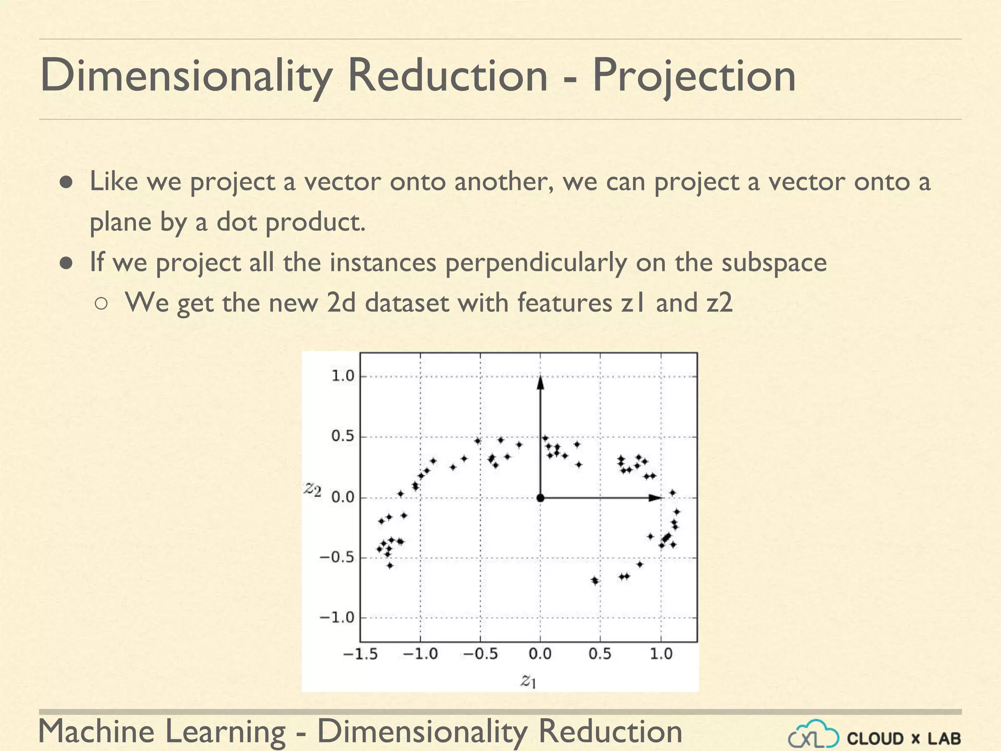
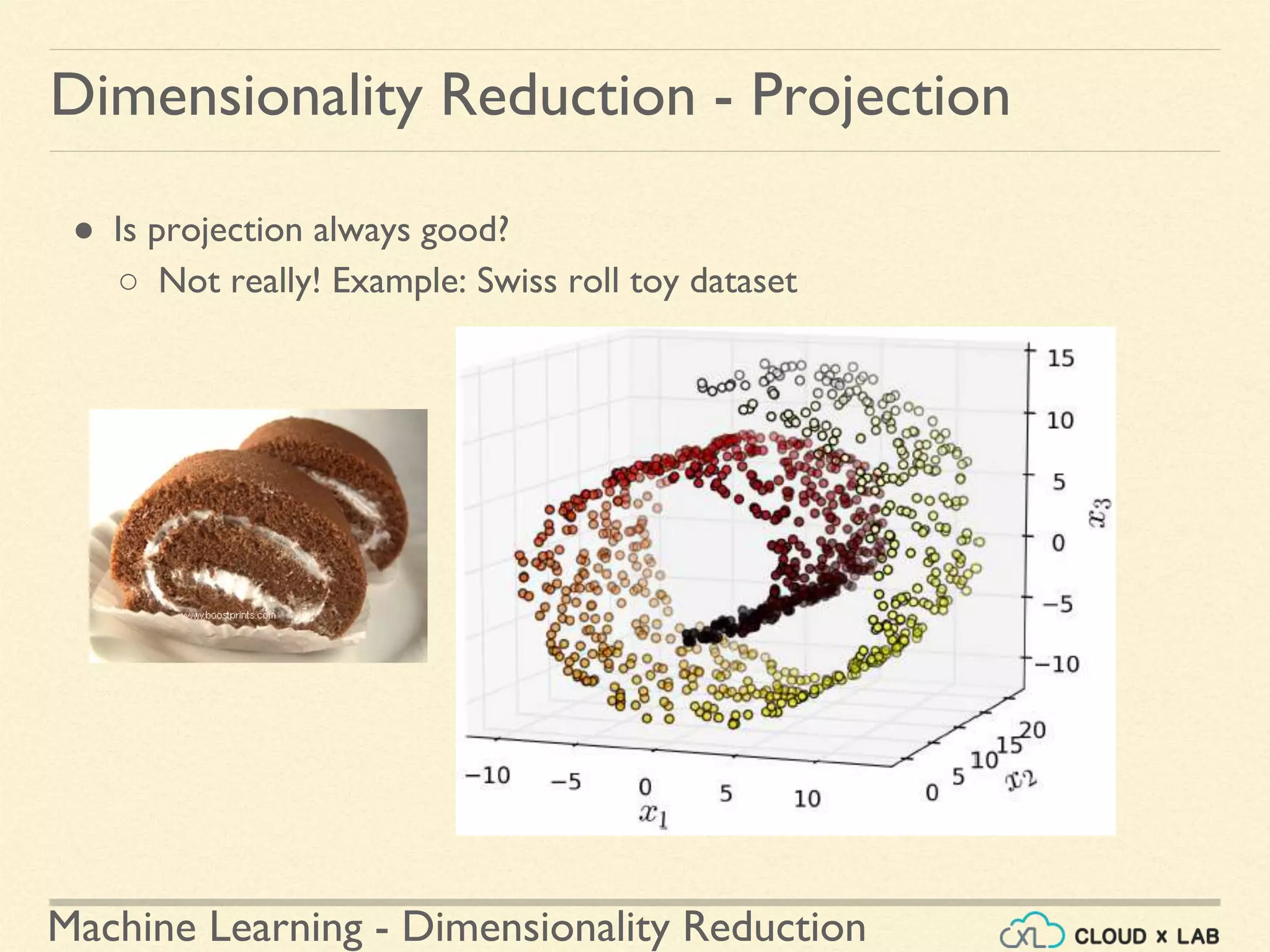
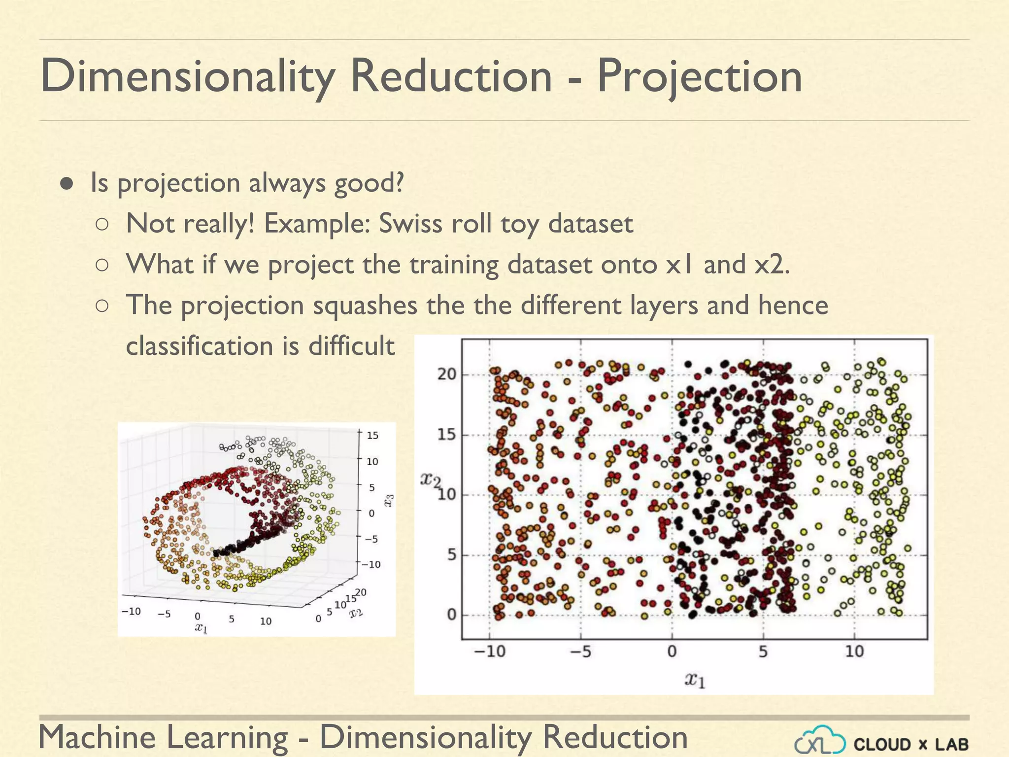
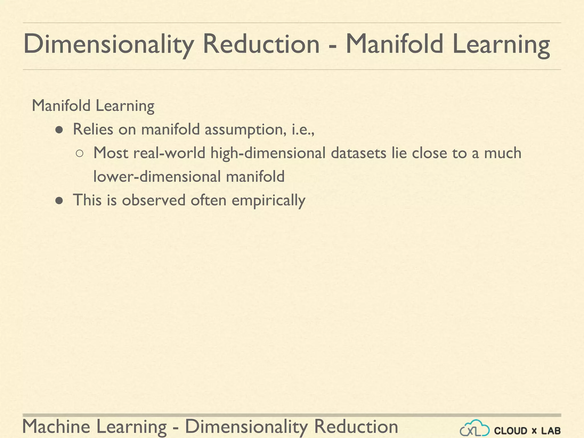
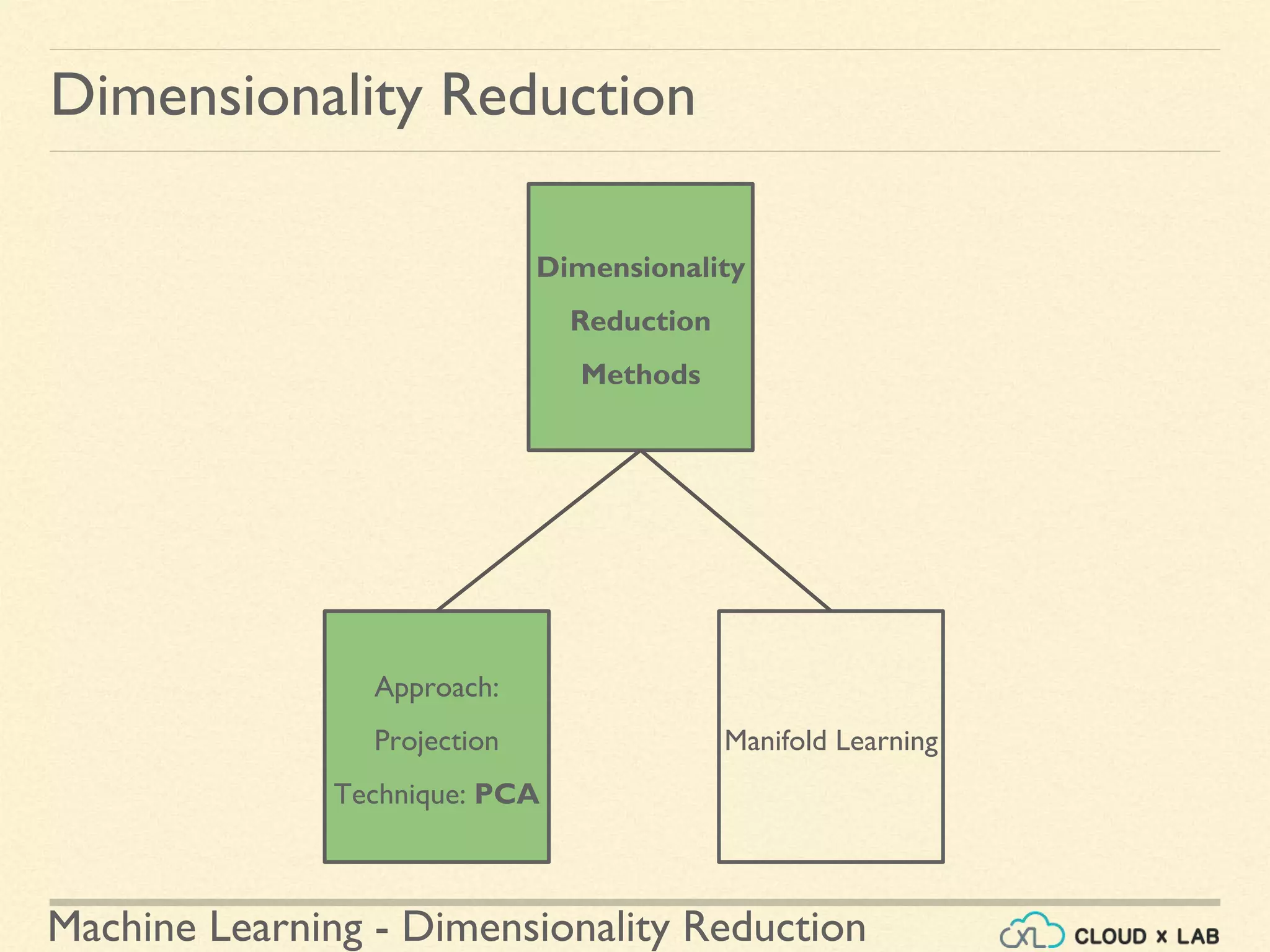
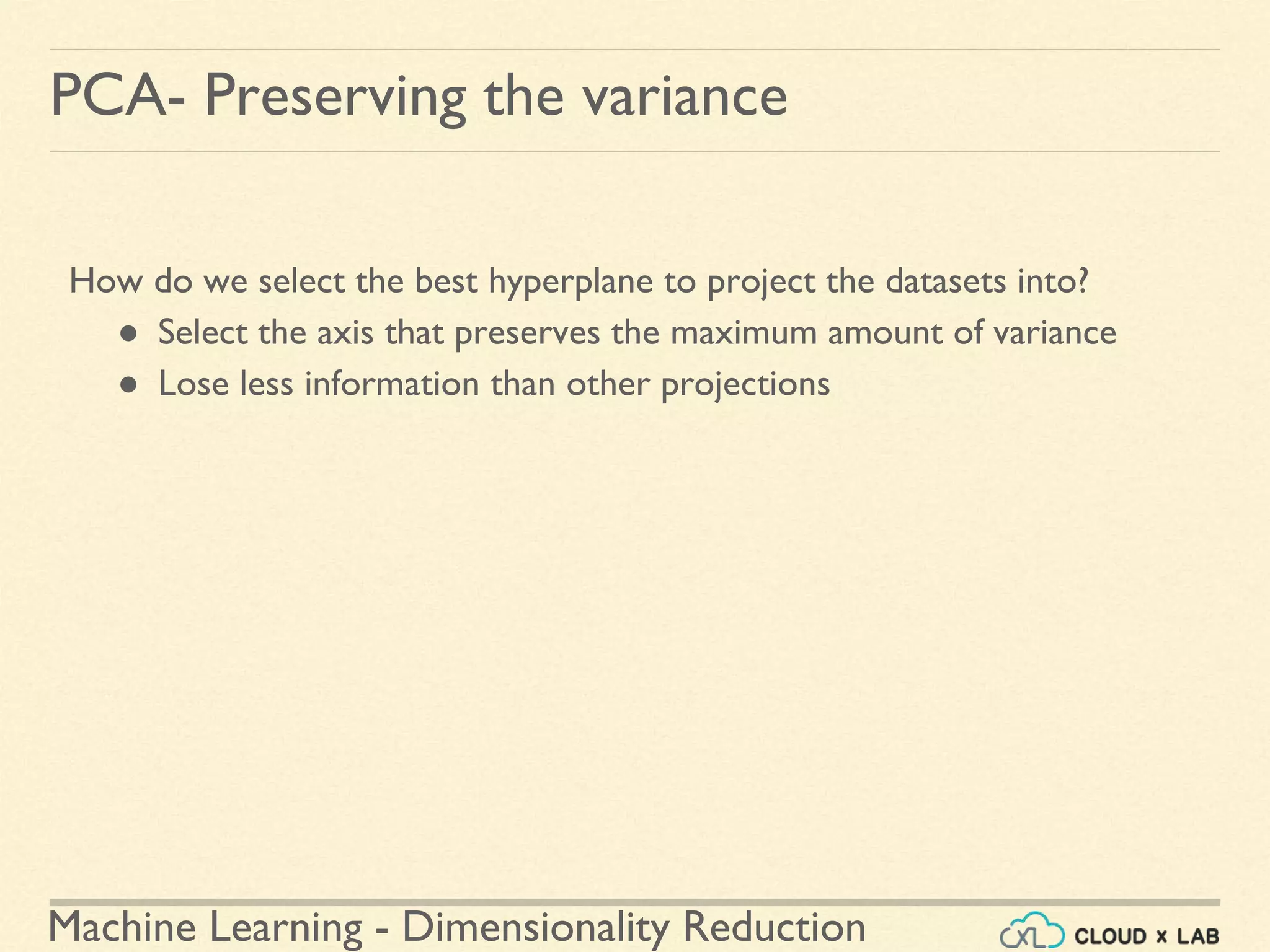
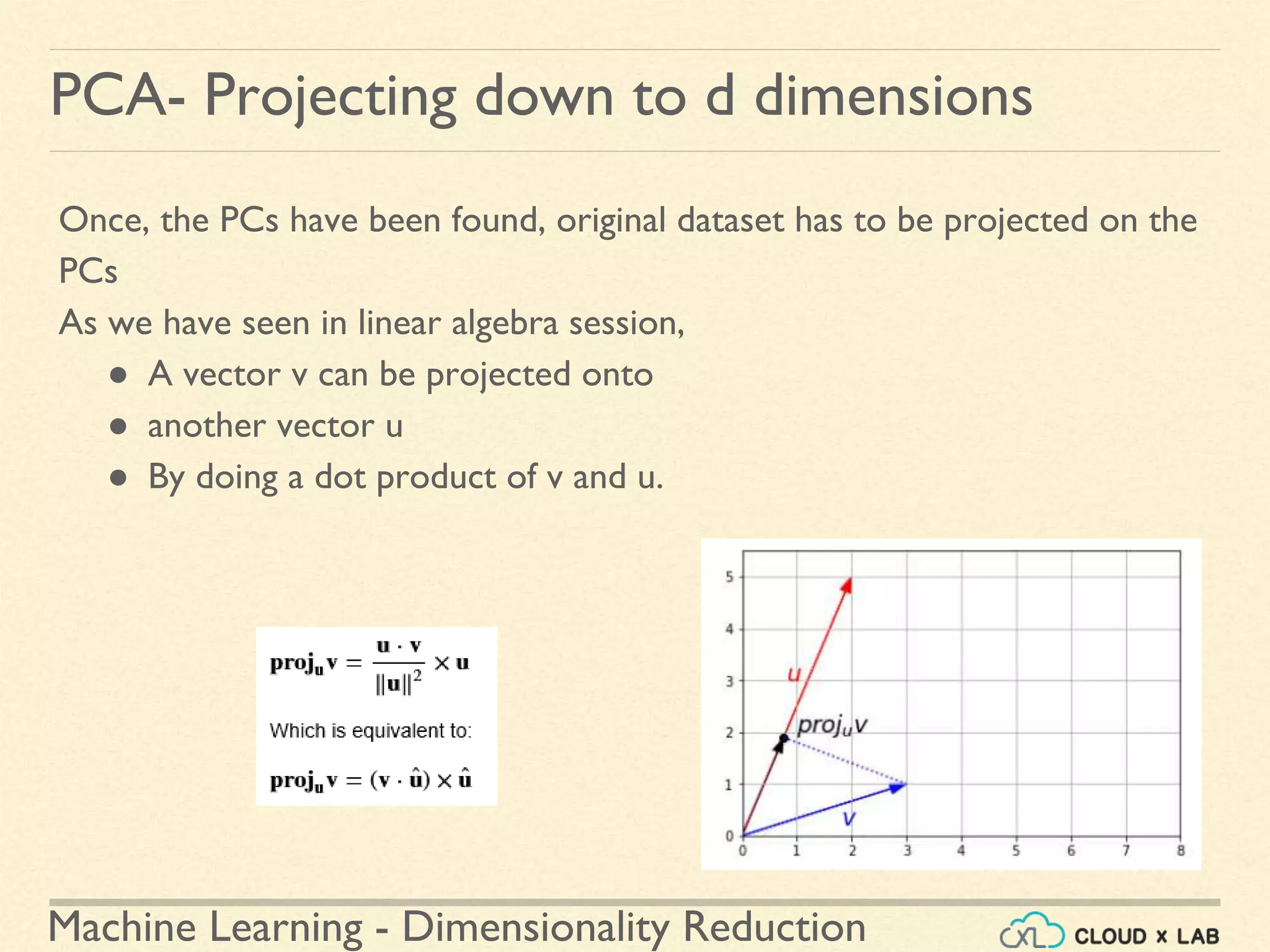
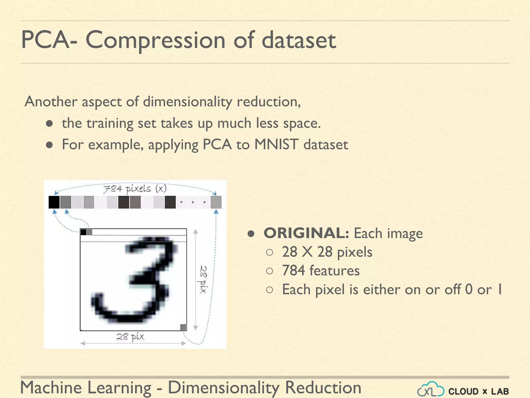
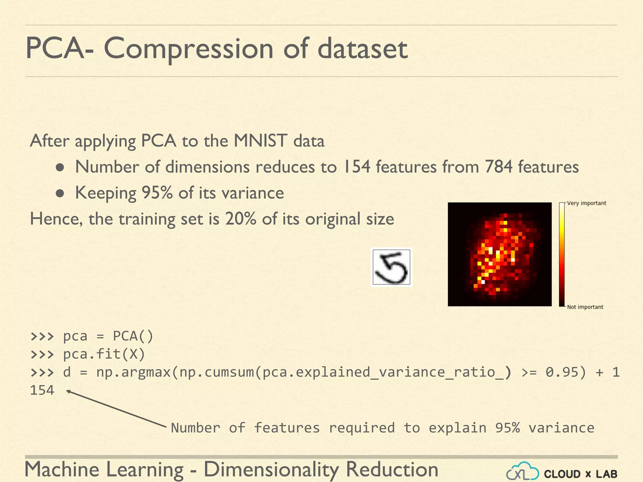
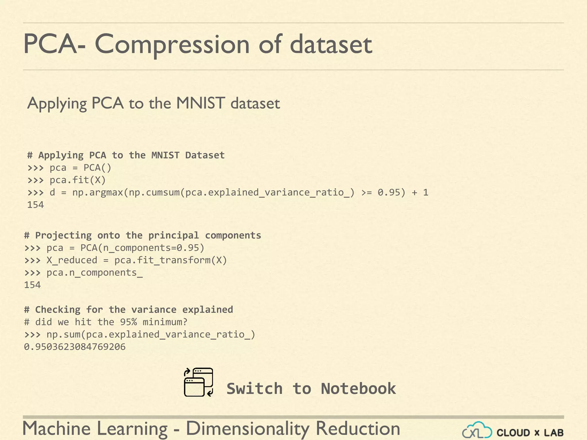
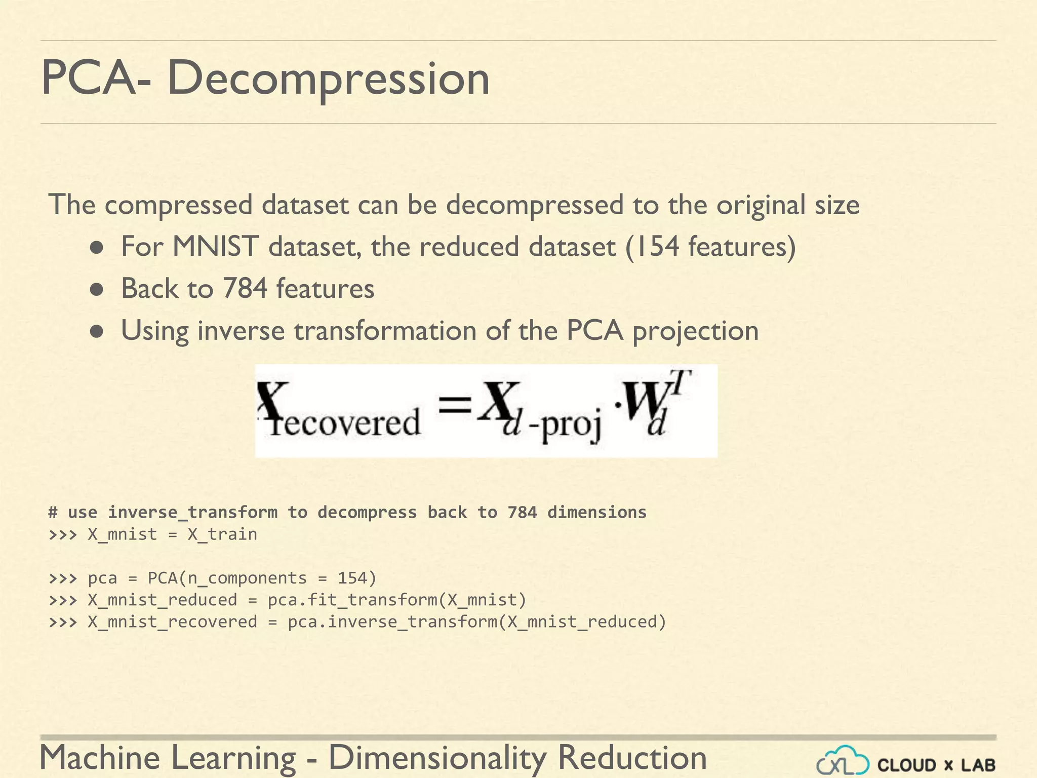
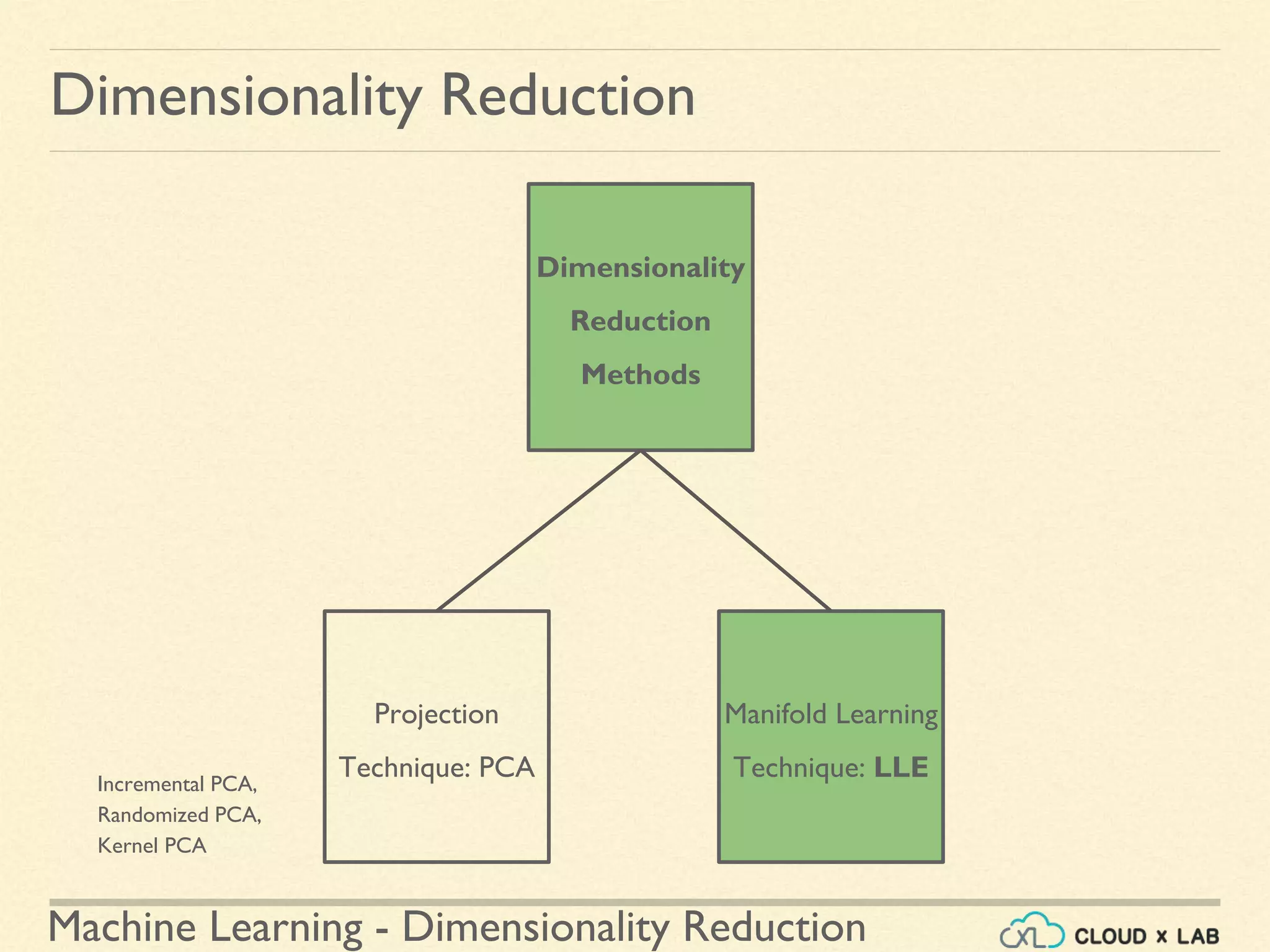
The document discusses dimensionality reduction in machine learning, explaining the curse of dimensionality and its negative impacts on model training and generalization. It introduces two main methods for dimensionality reduction: projection and manifold learning, detailing their benefits and potential drawbacks, such as information loss. The text also highlights PCA (Principal Component Analysis) as a popular algorithm for reducing dimensions while preserving variance.


![Dimension reduction techniques[Feature Selection]](https://cdn.slidesharecdn.com/ss_thumbnails/dimensionreductiontechnibyaakankshajain-210625102243-thumbnail.jpg?width=640&height=640&fit=bounds)