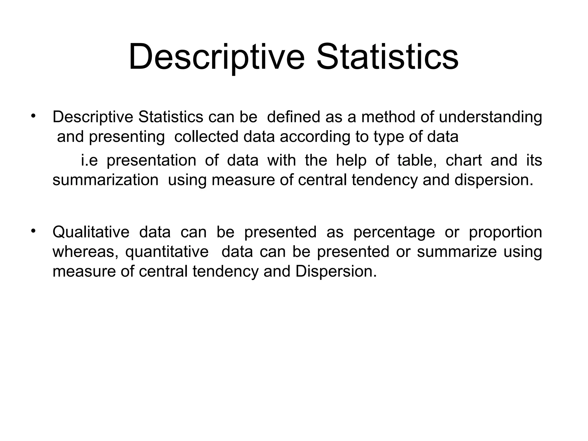
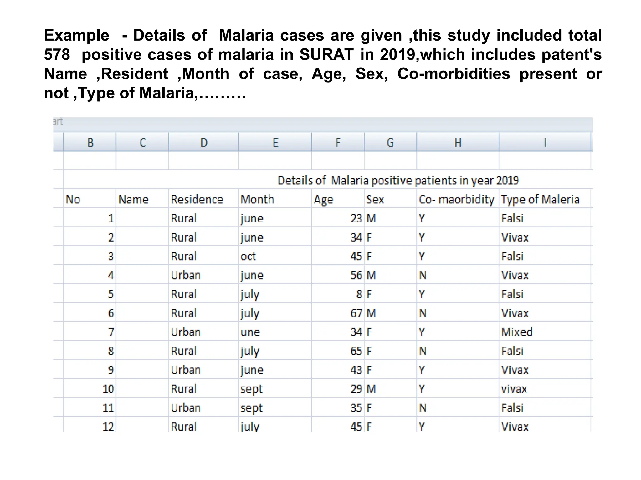
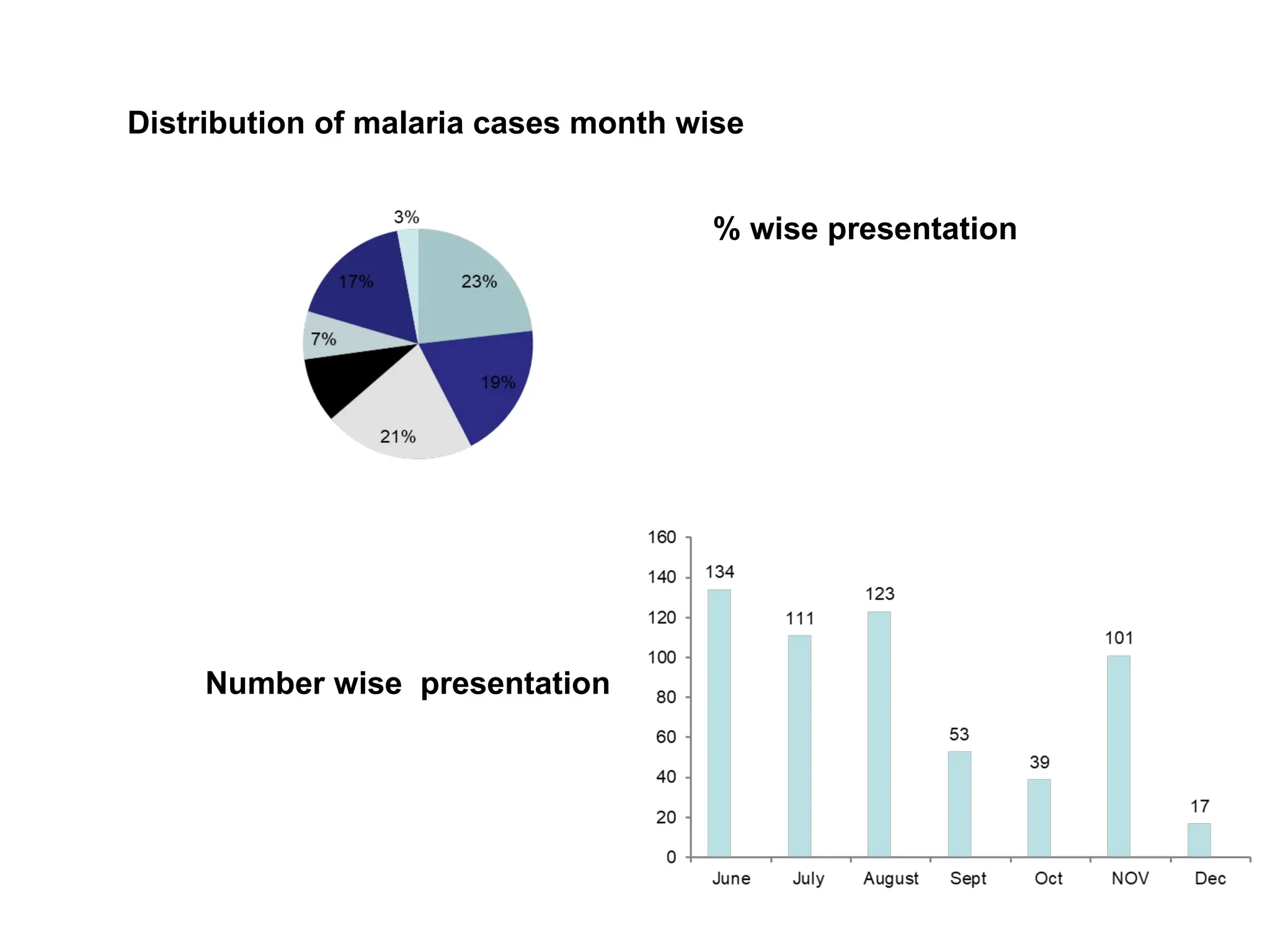
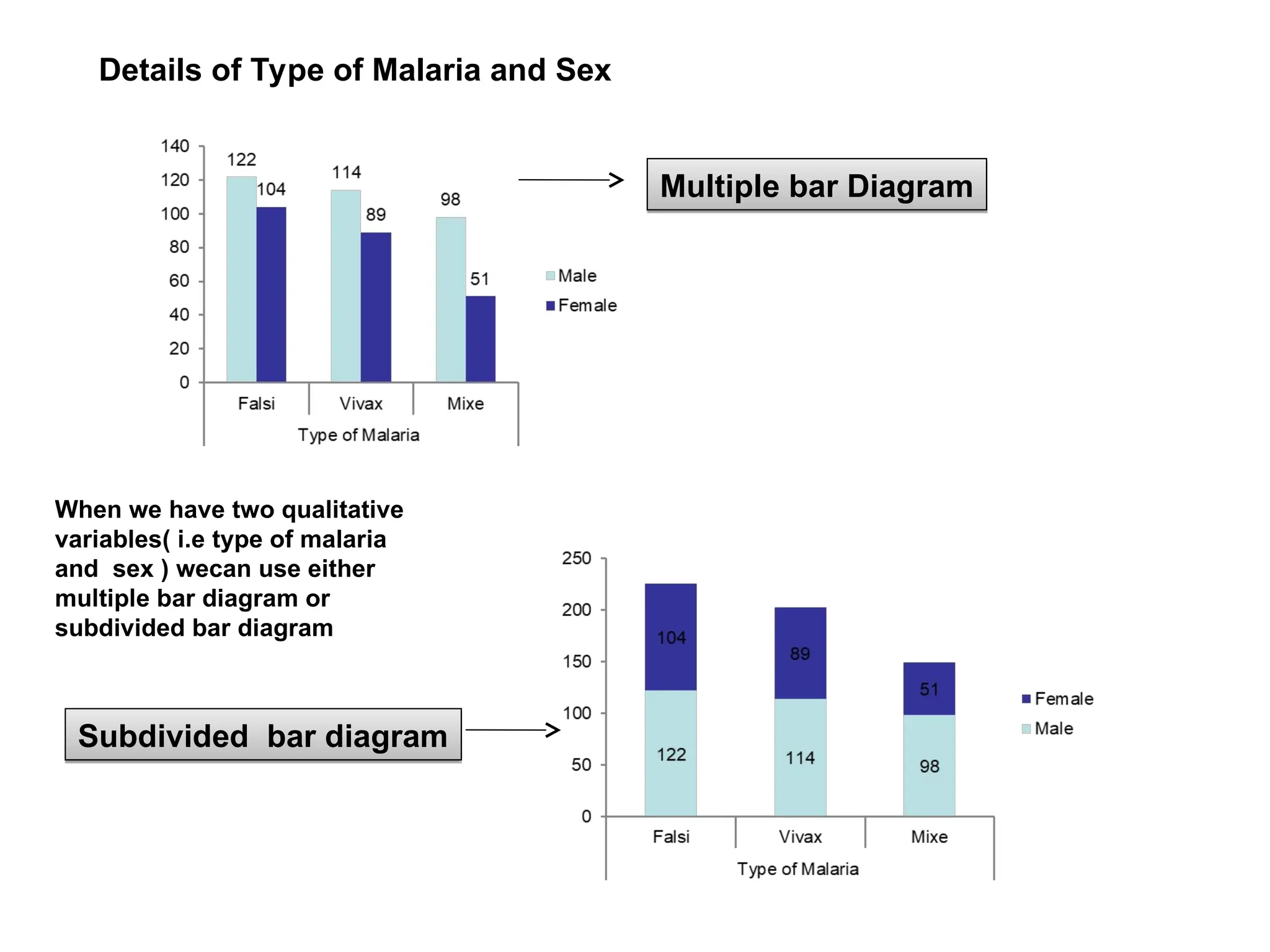
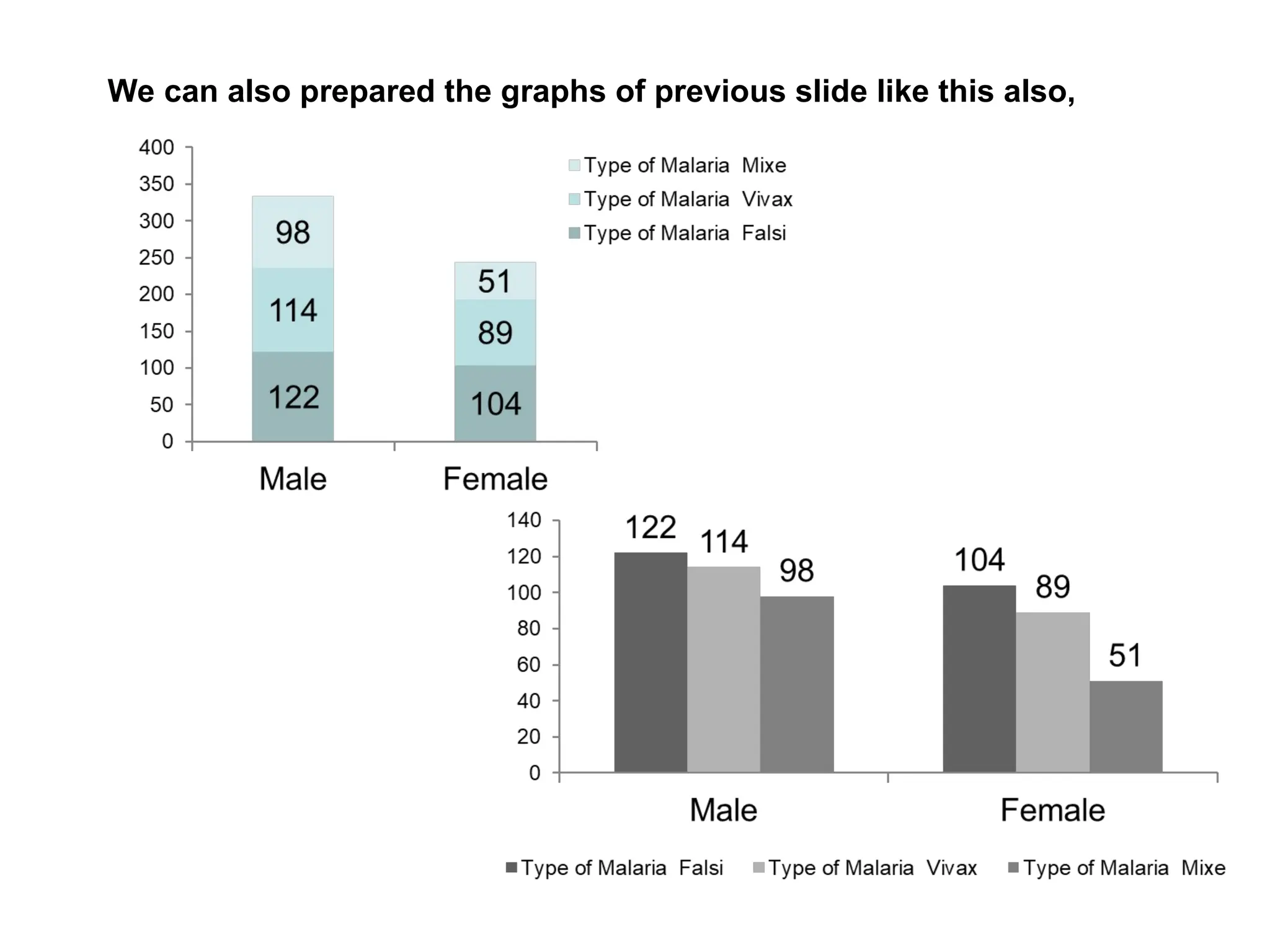
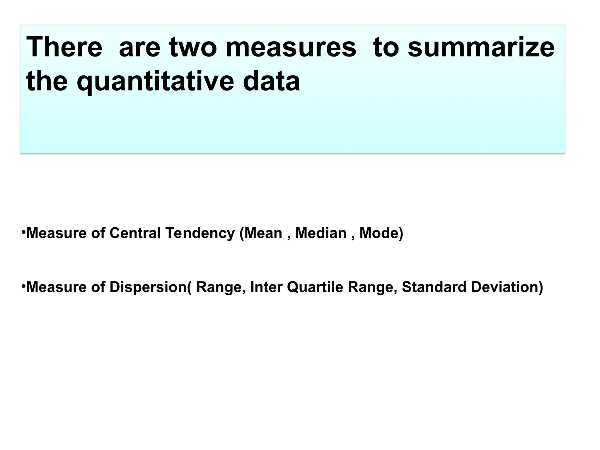
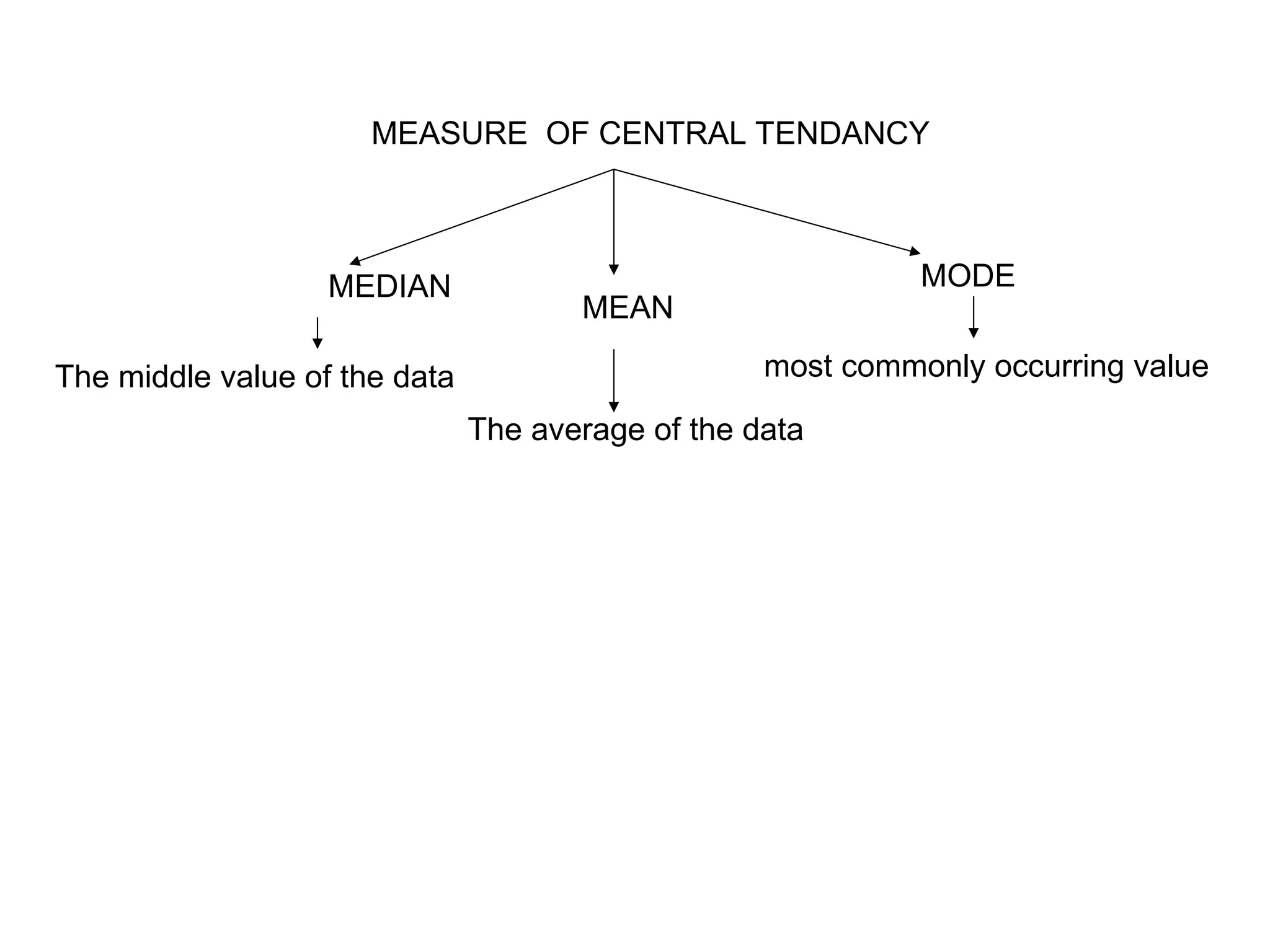
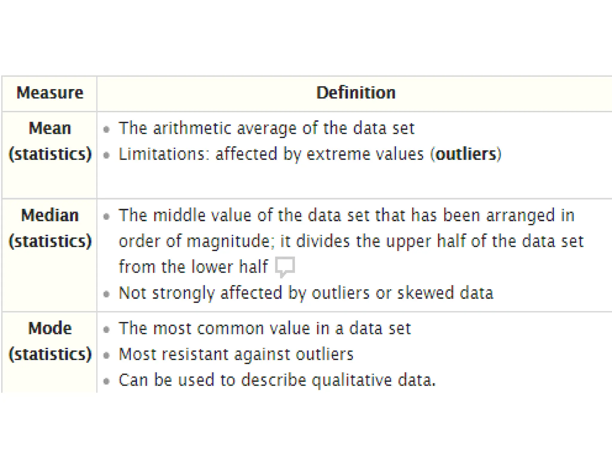
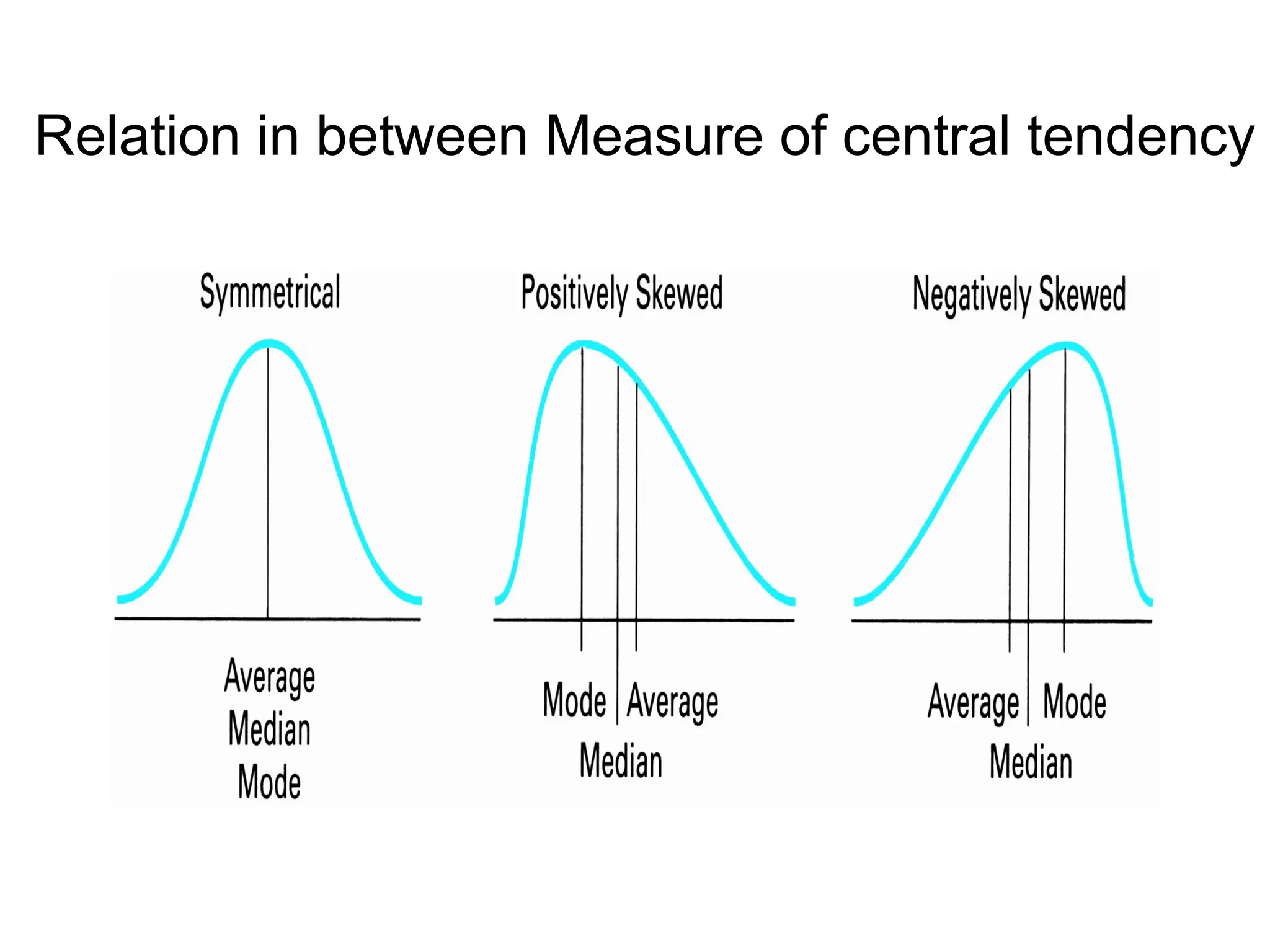
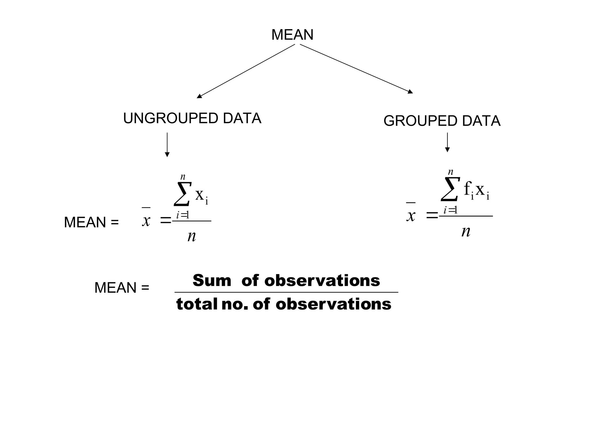
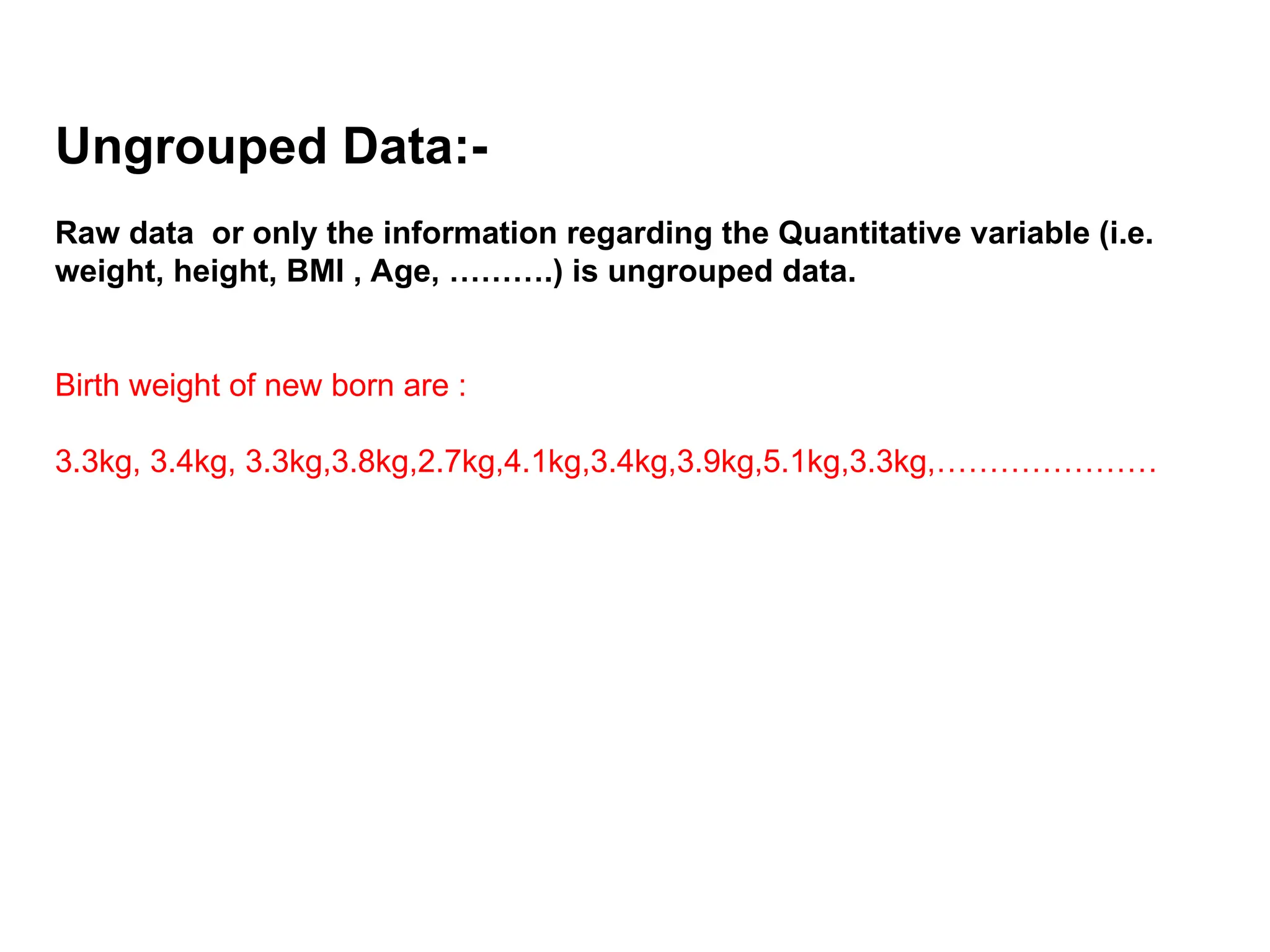
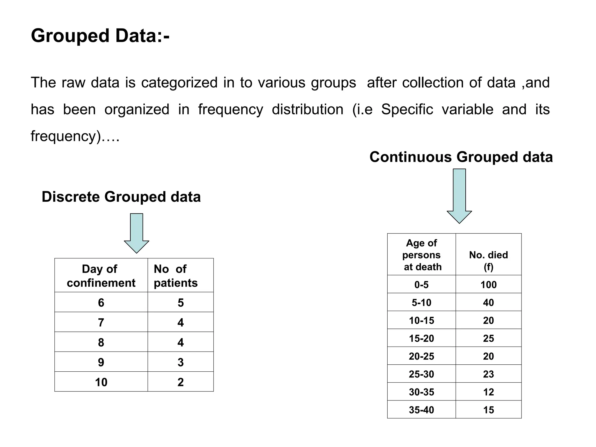
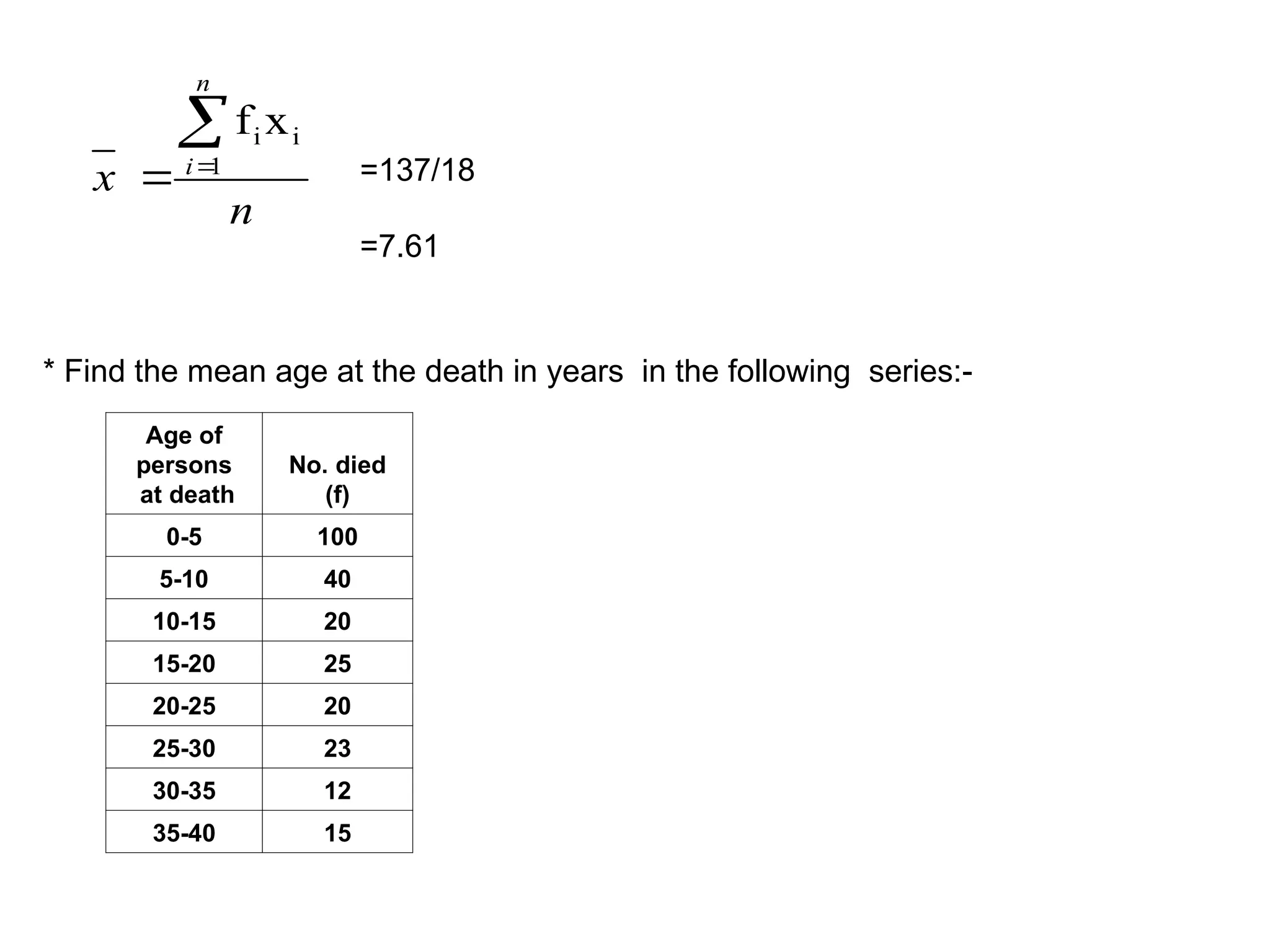
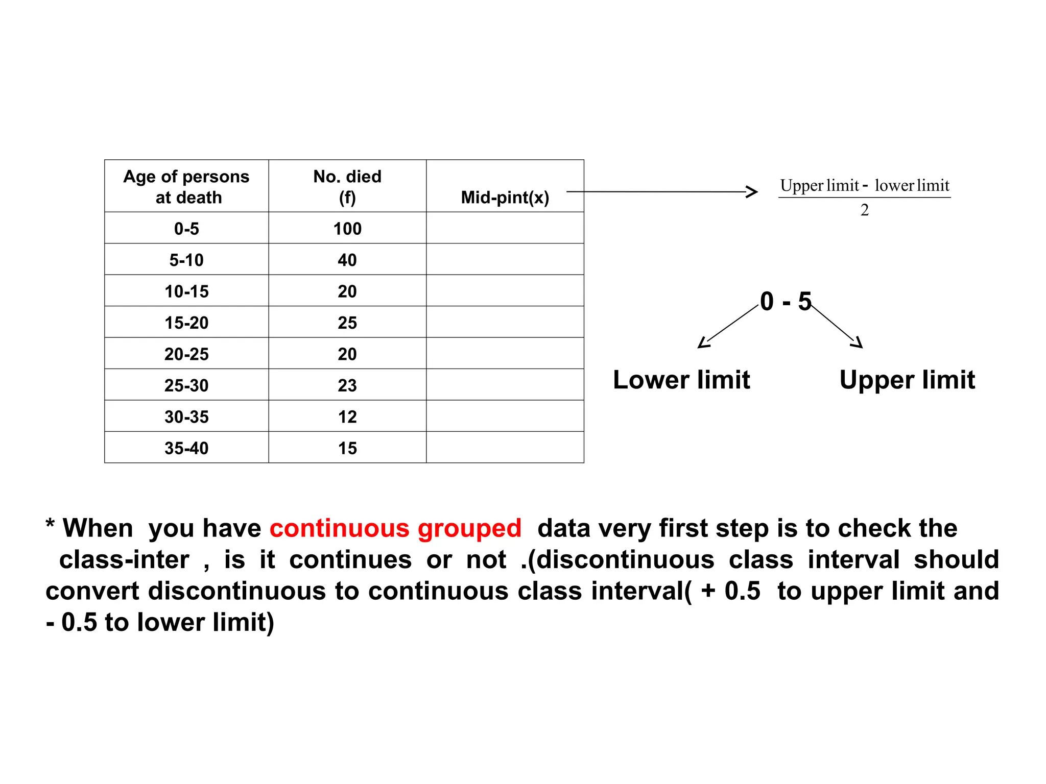
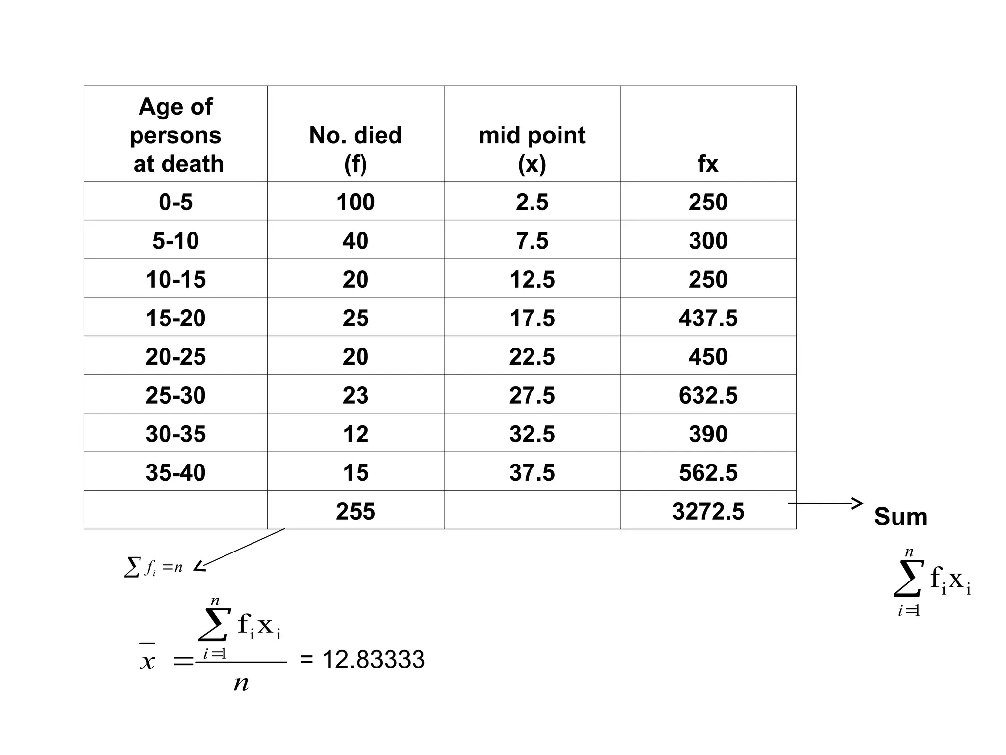
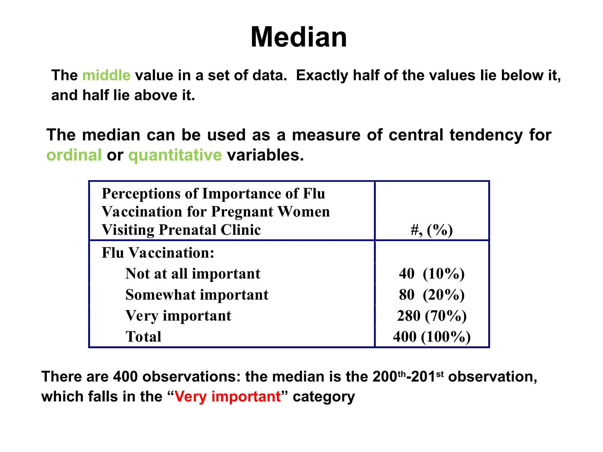
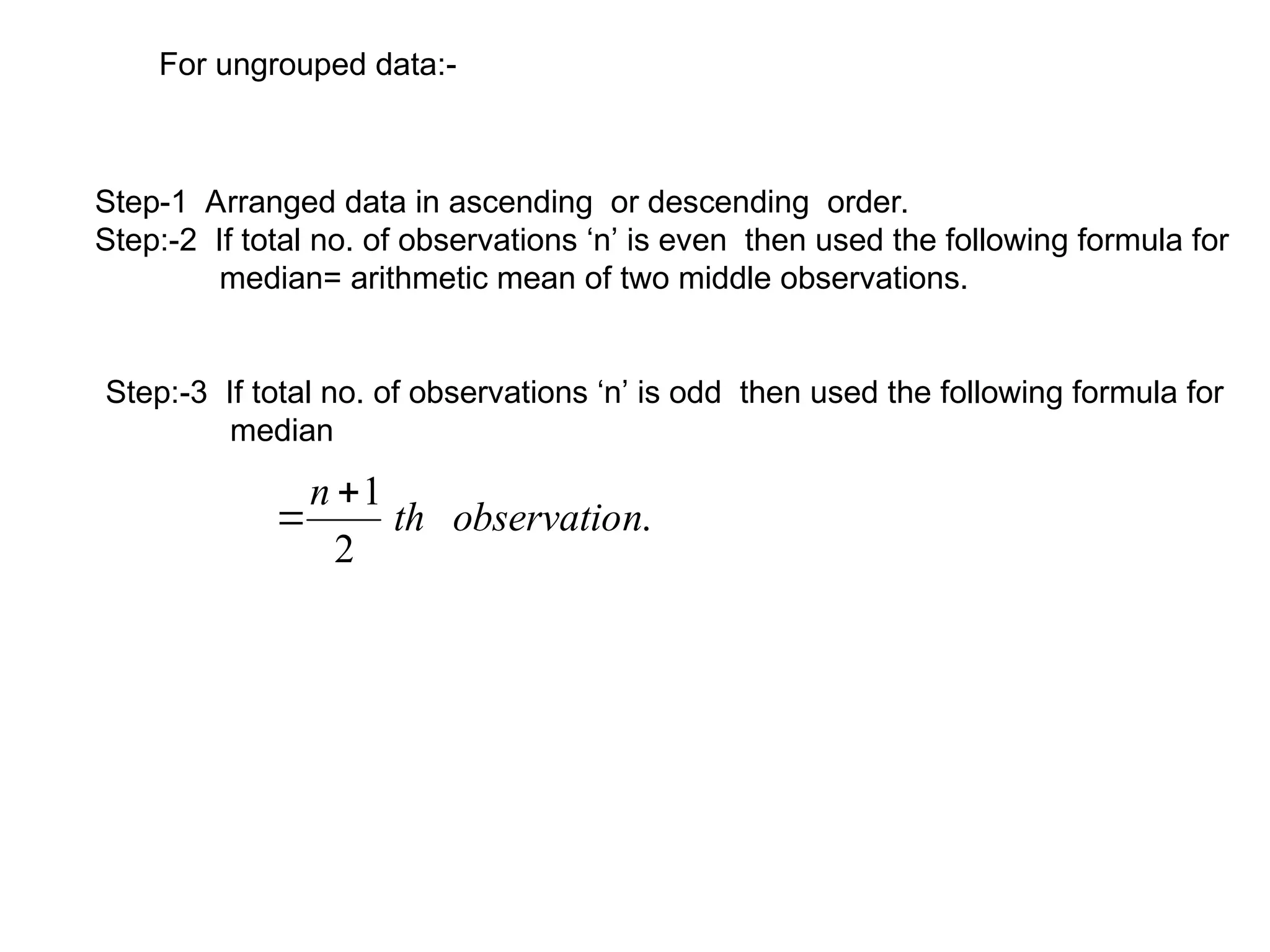
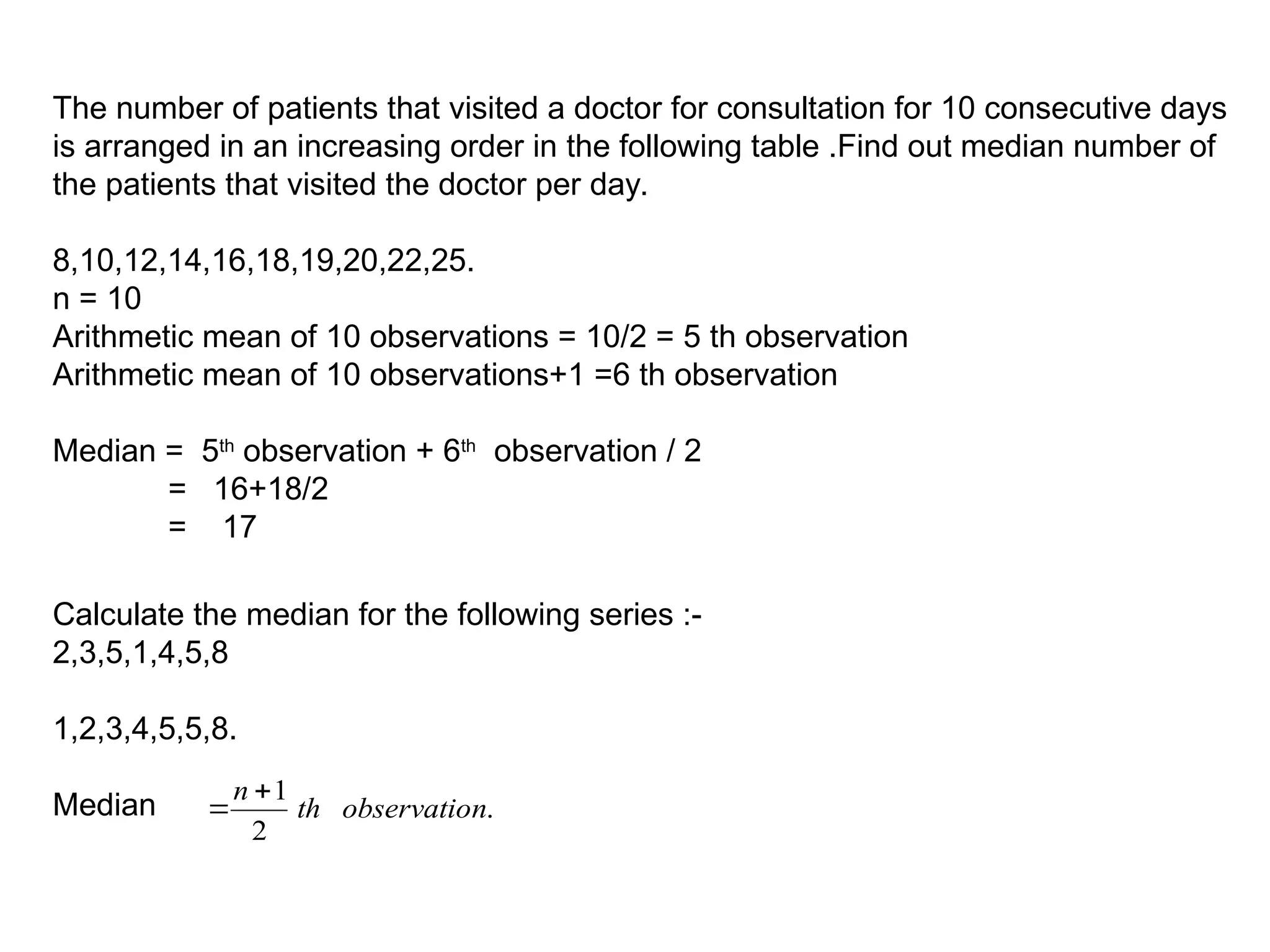
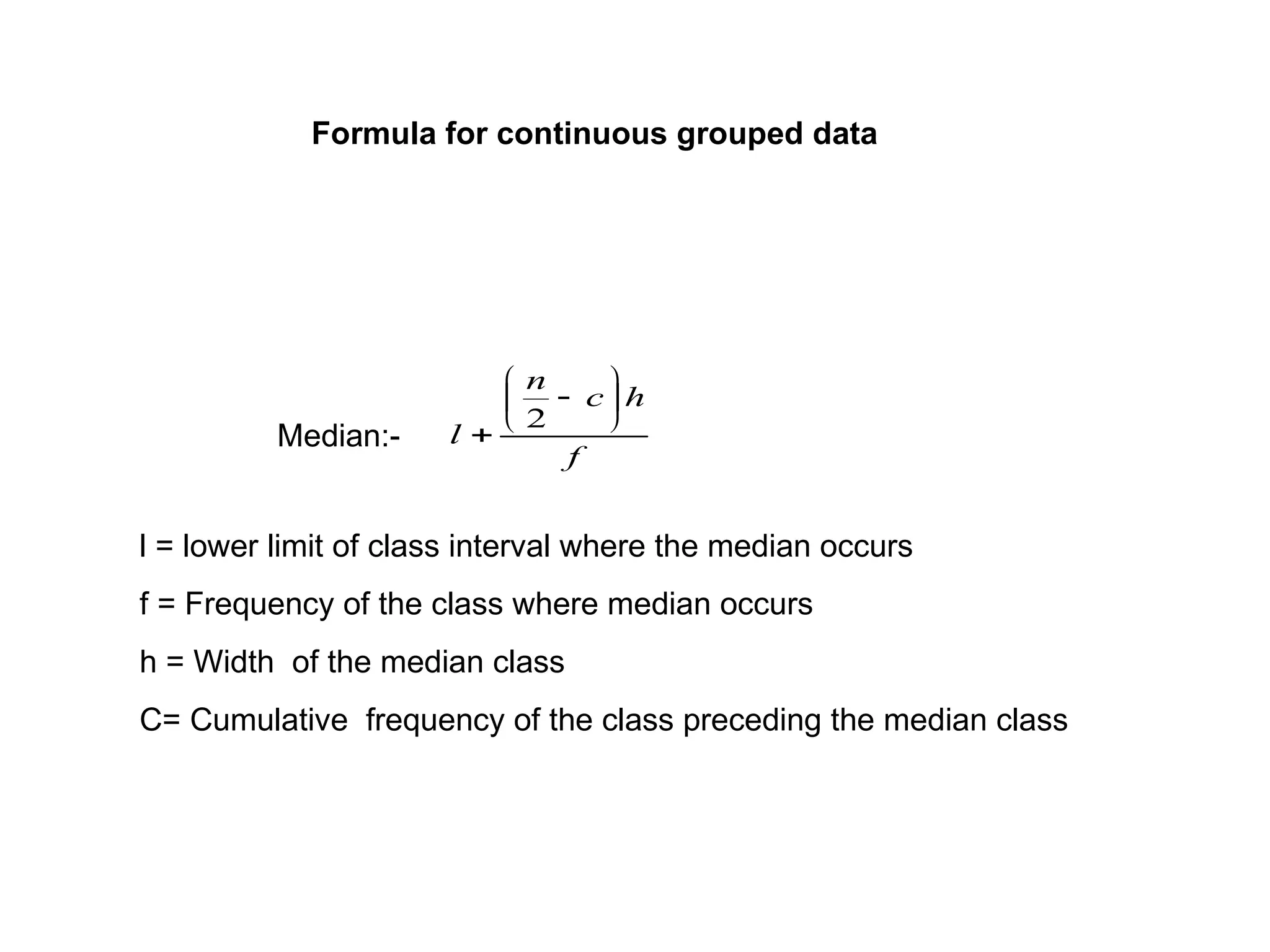
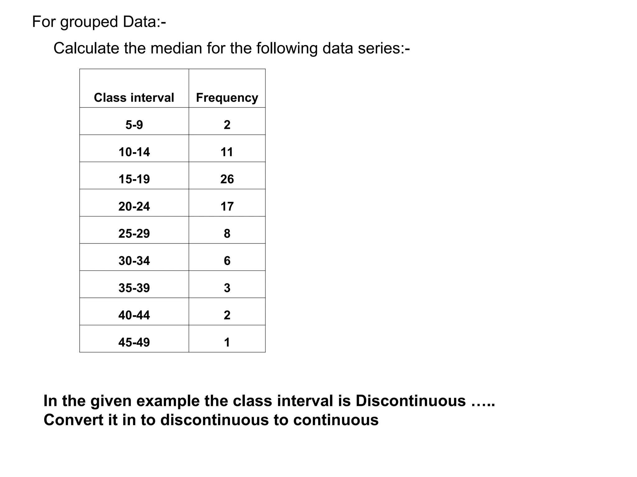
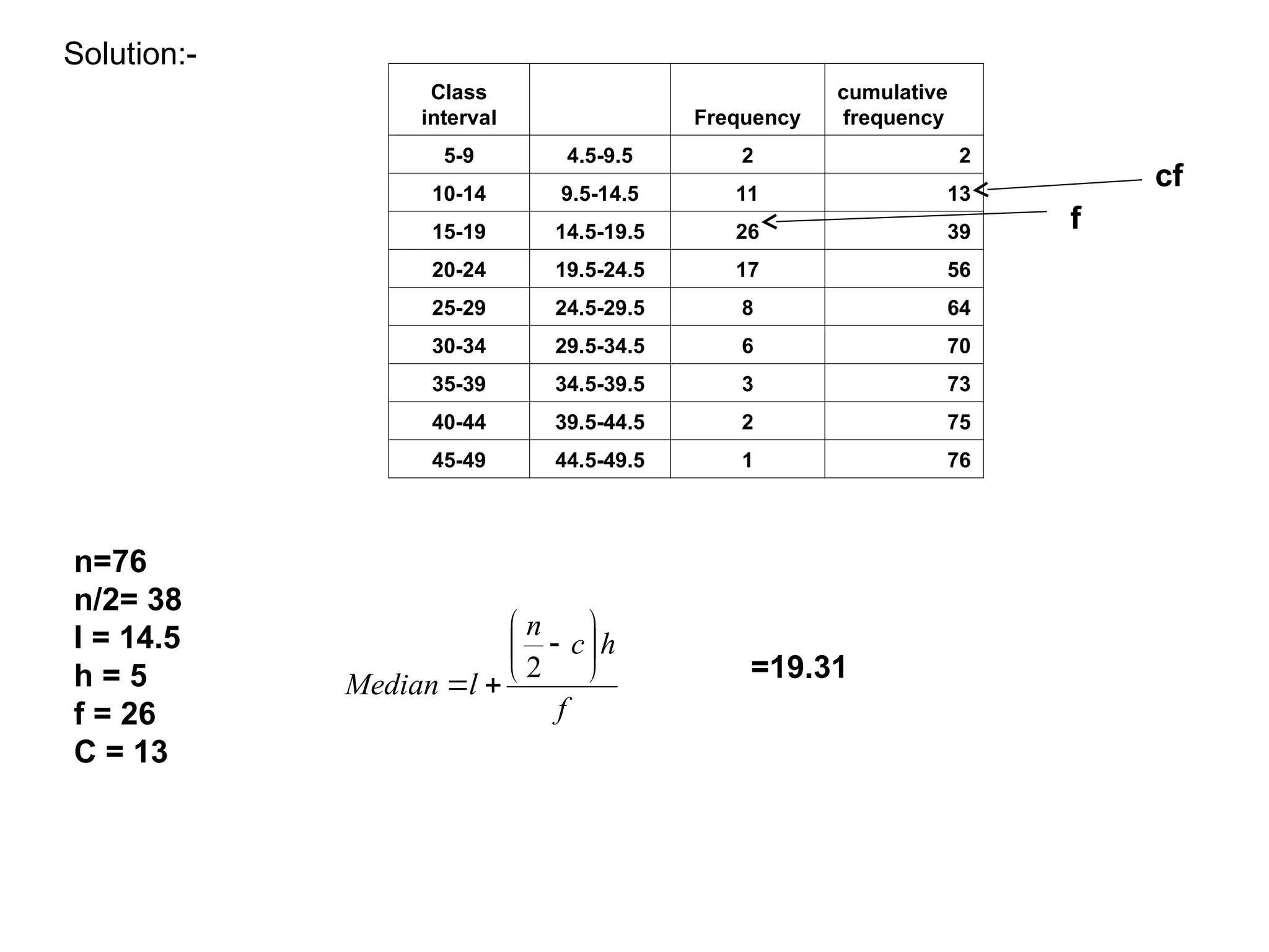
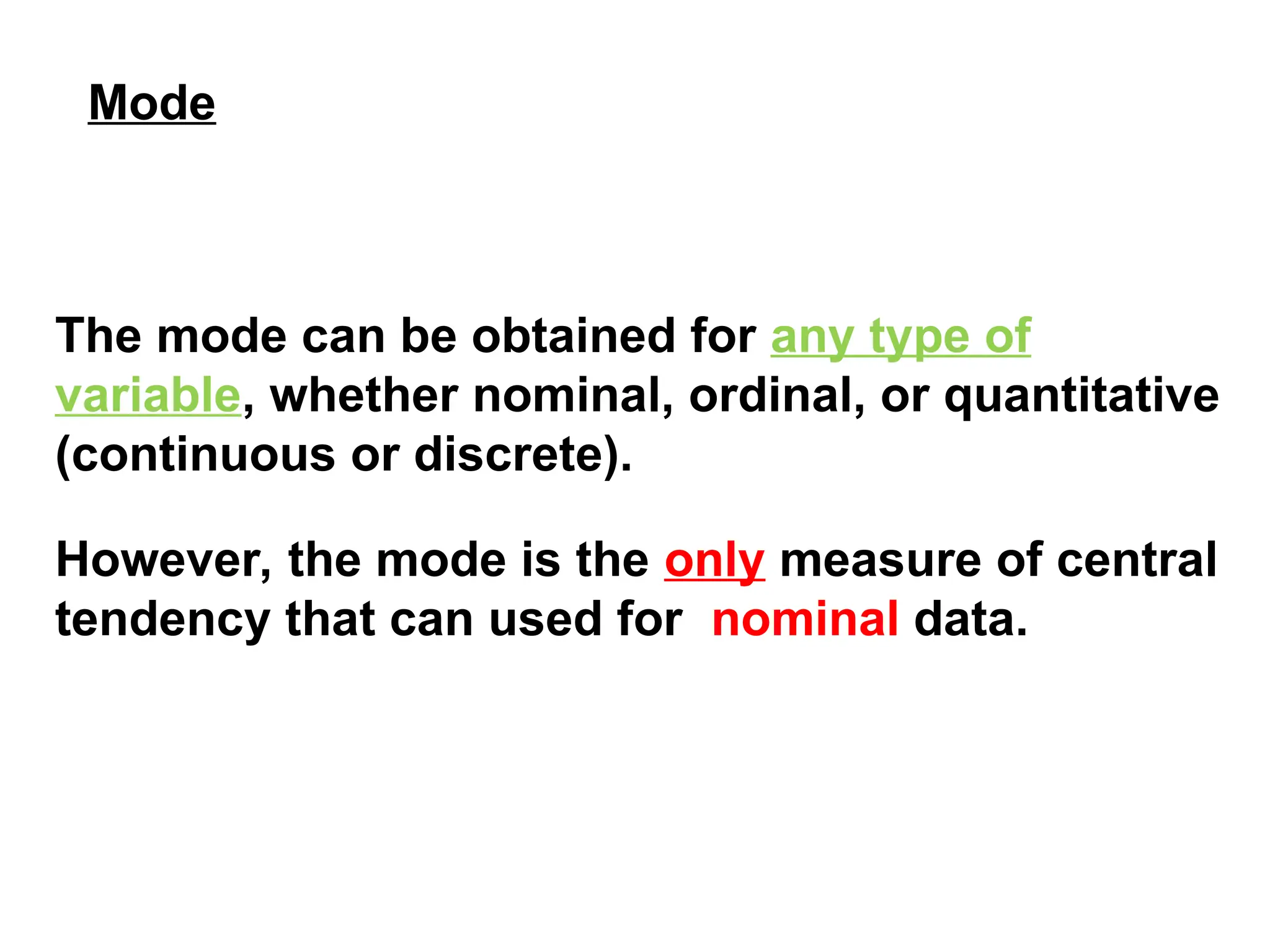
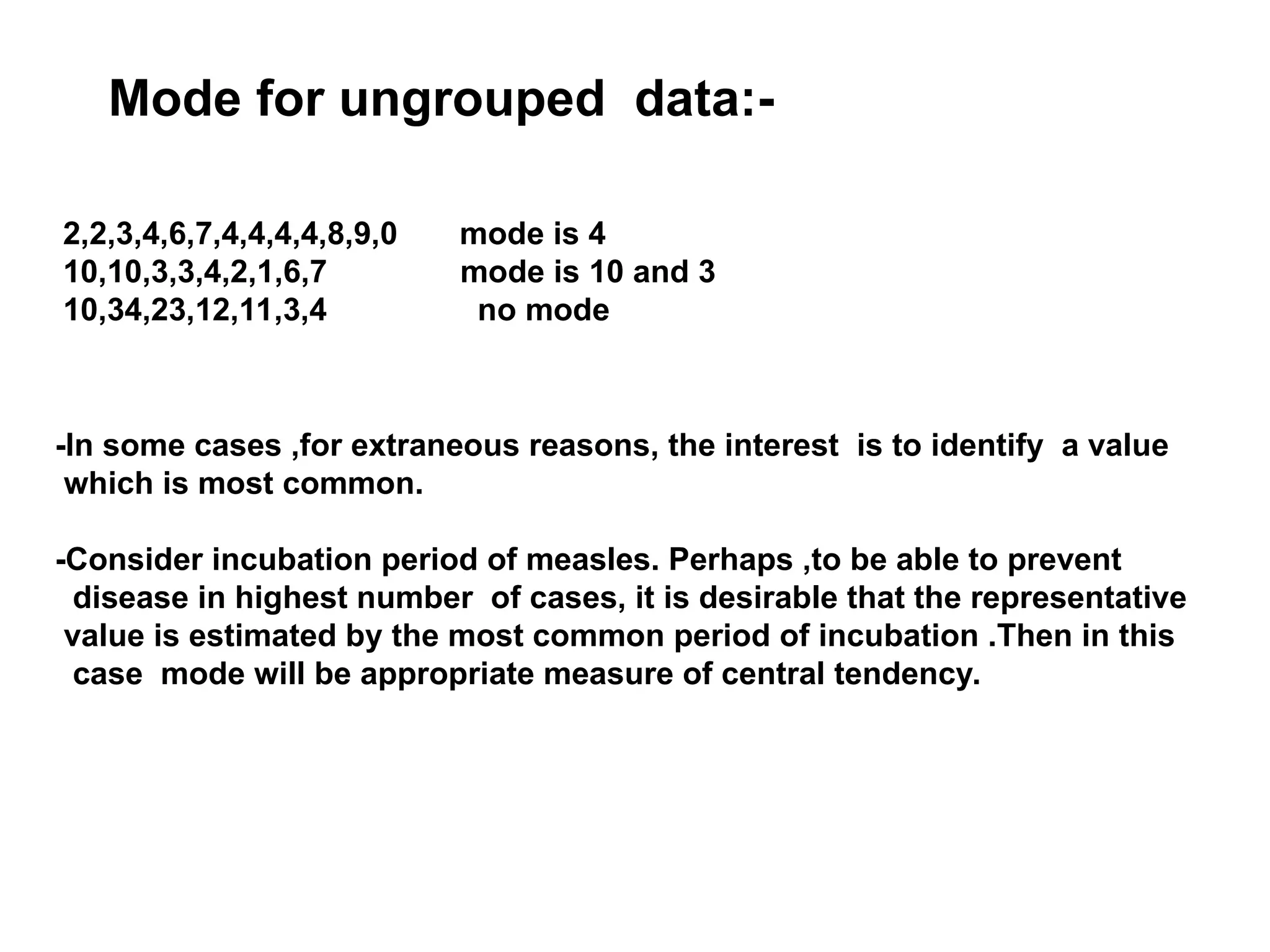
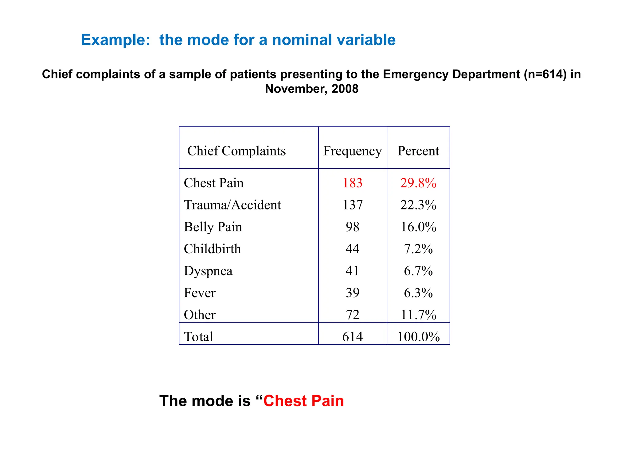
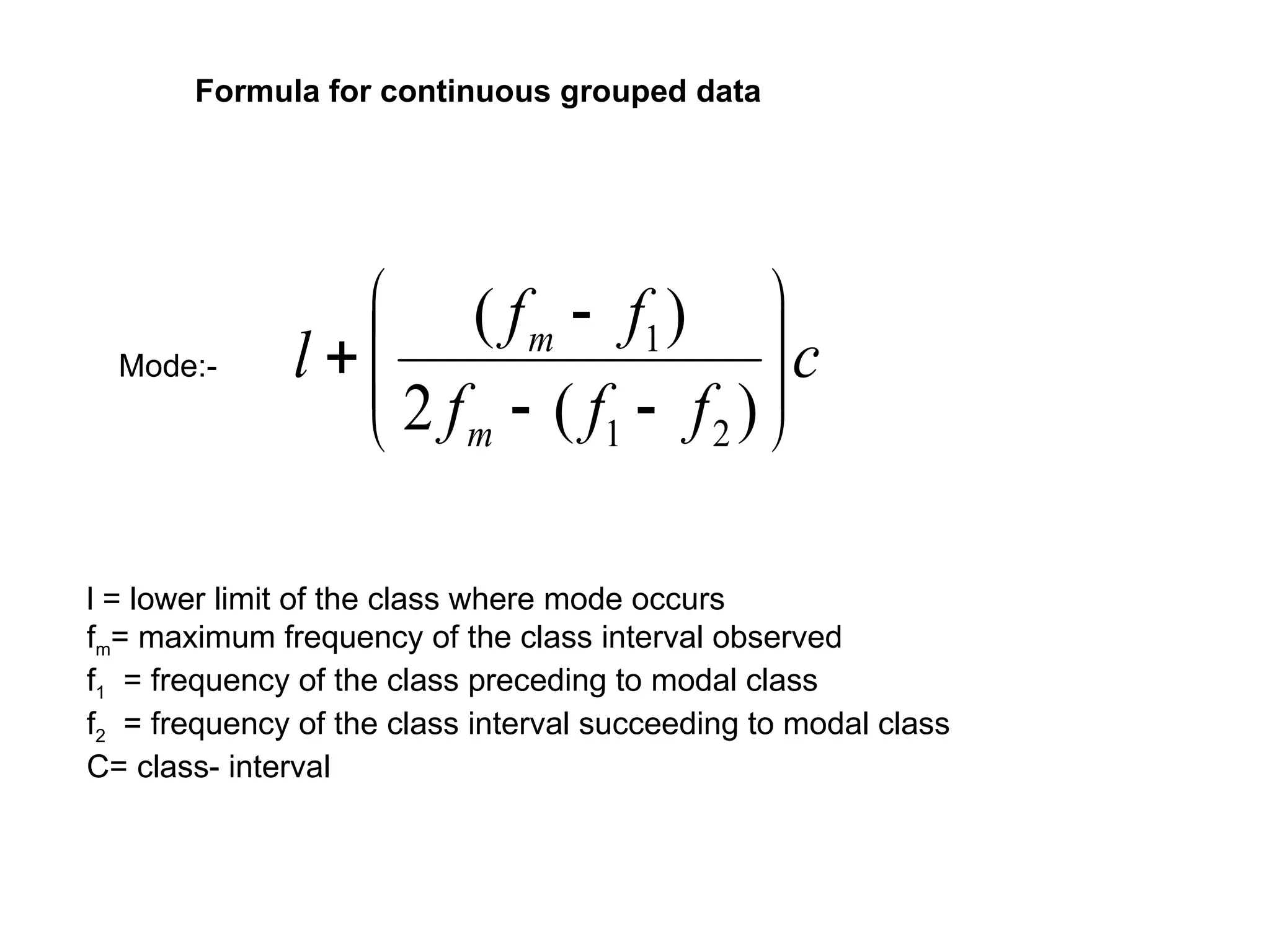
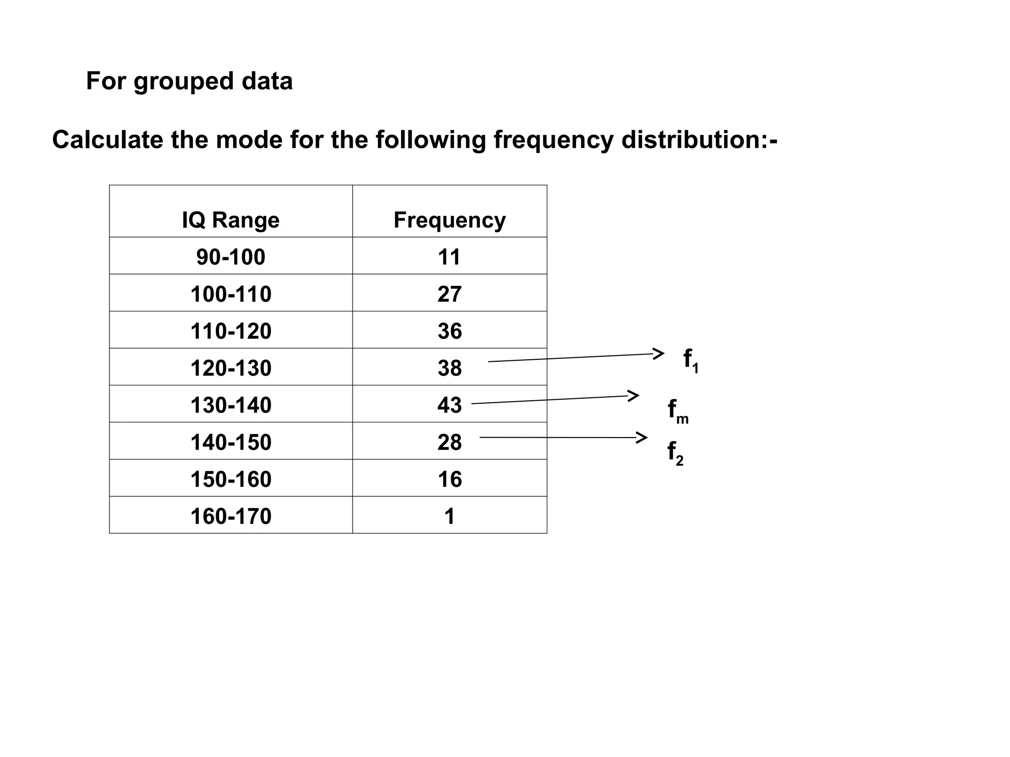
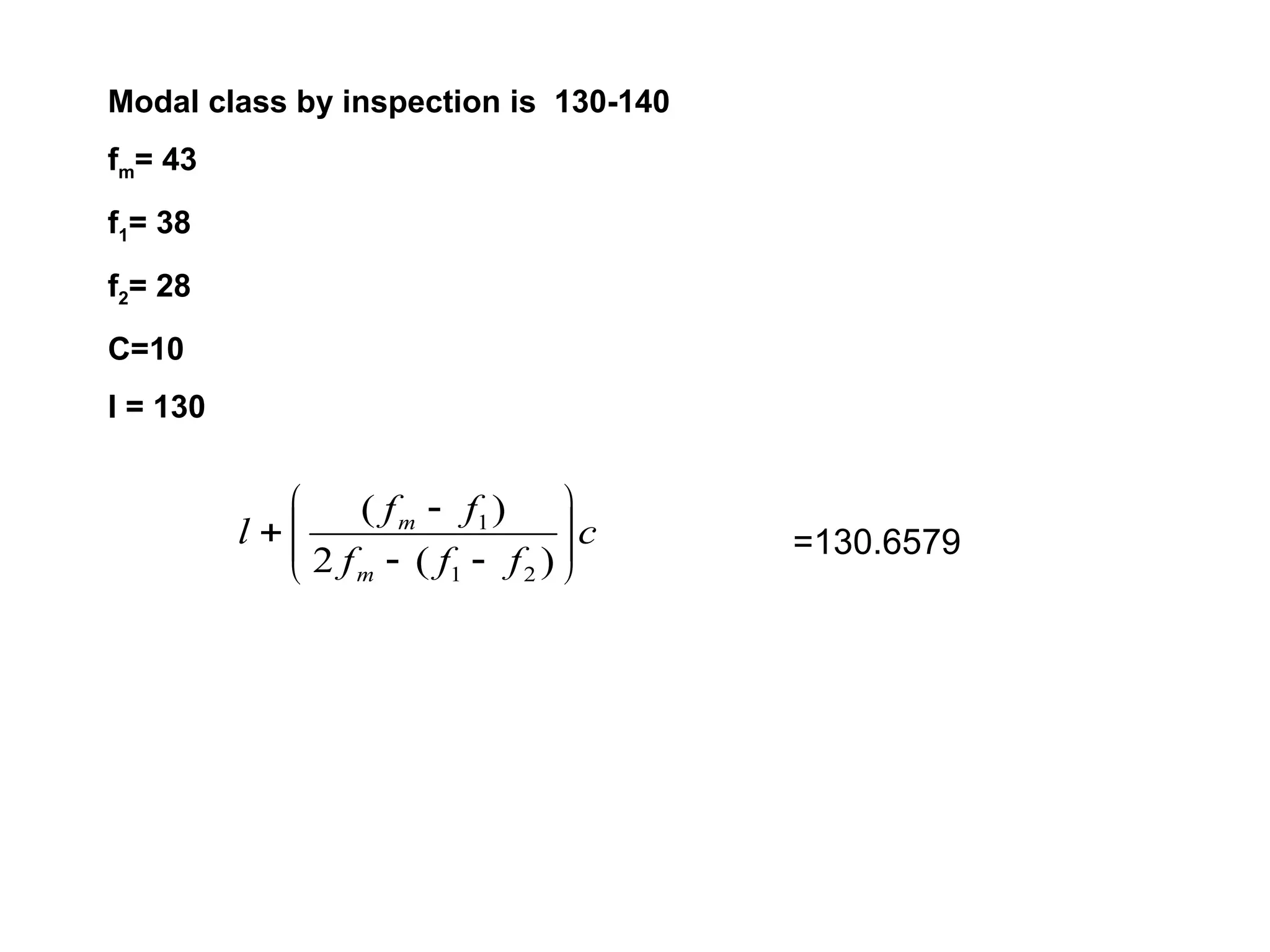
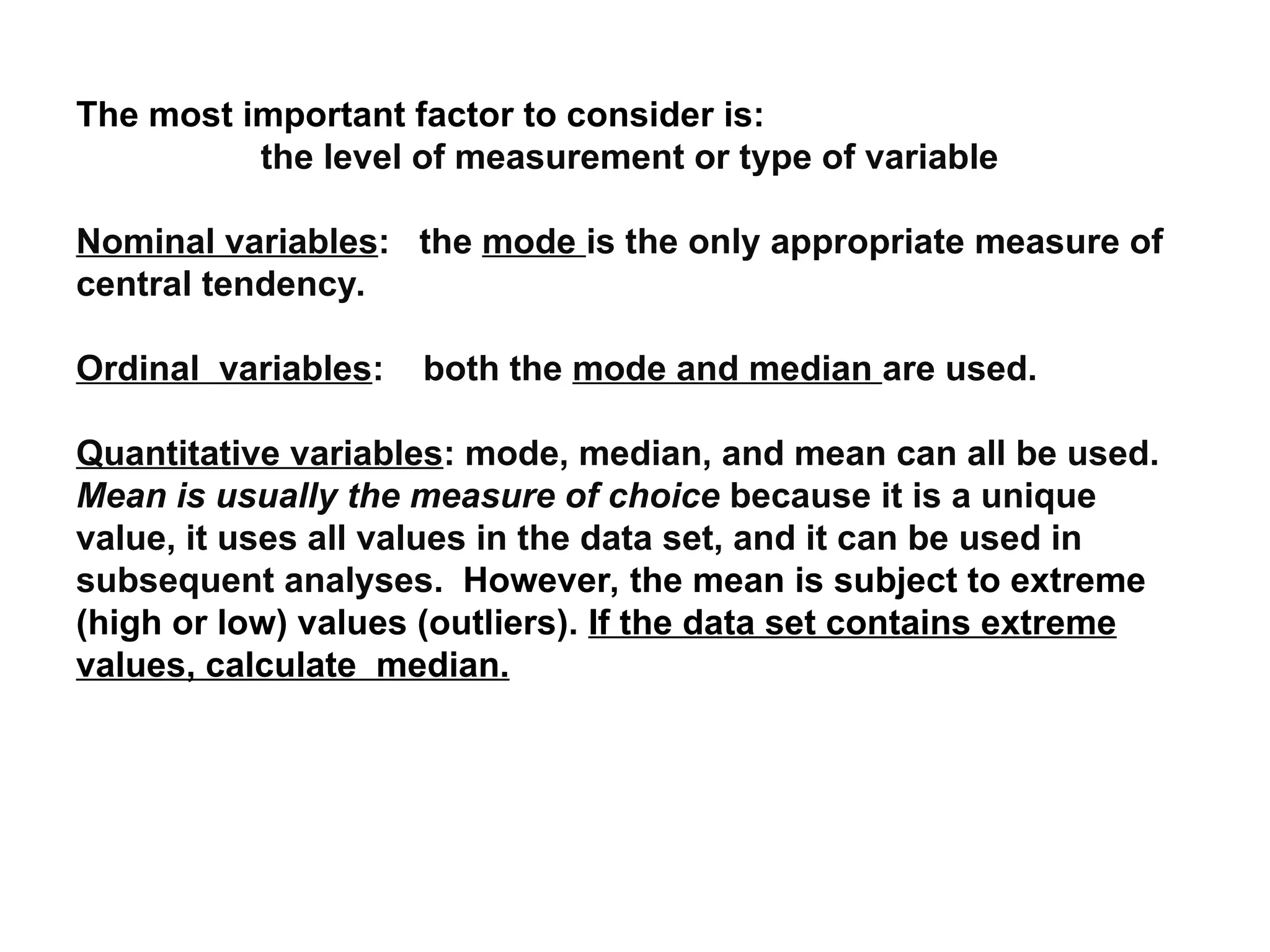
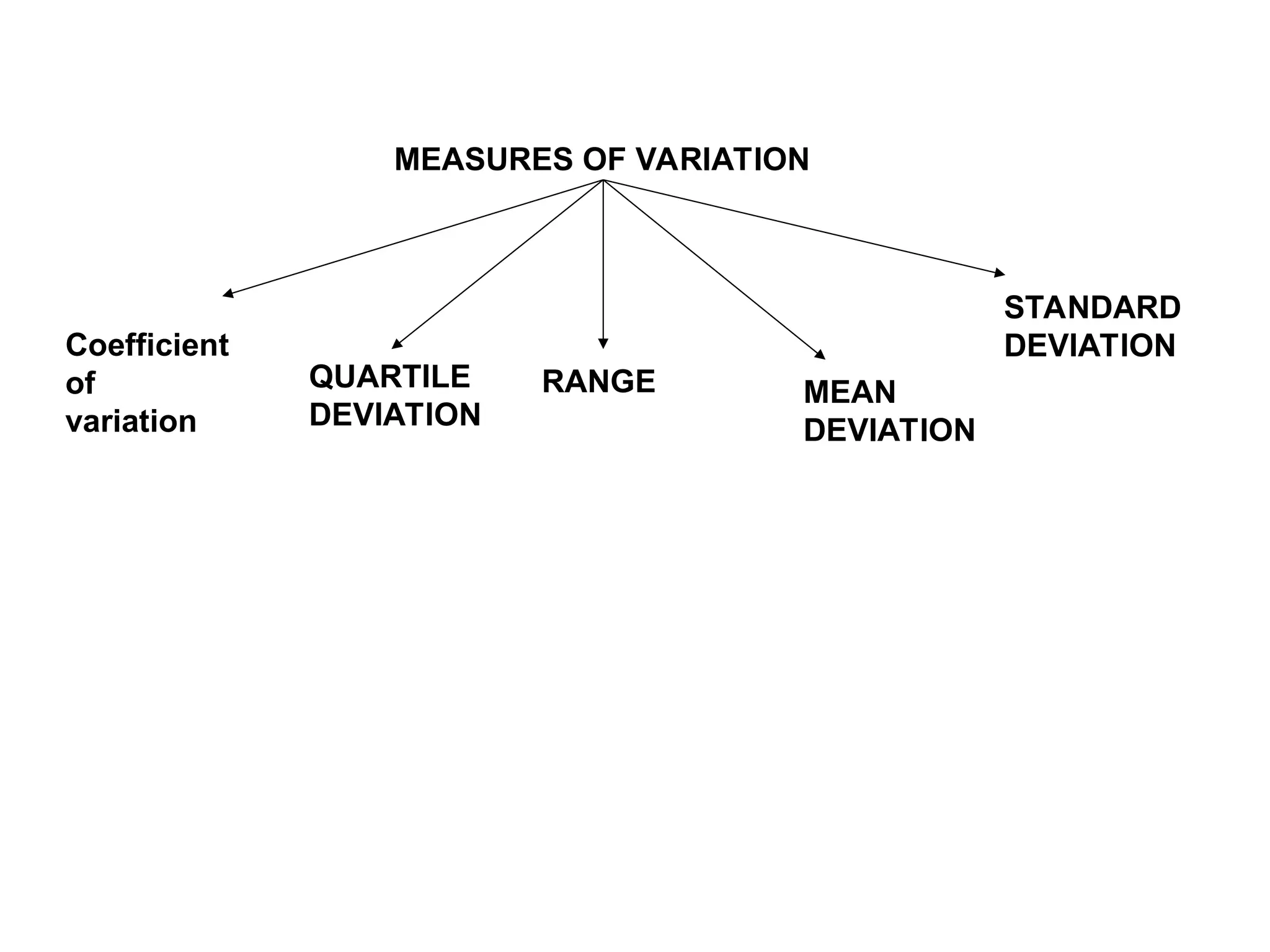
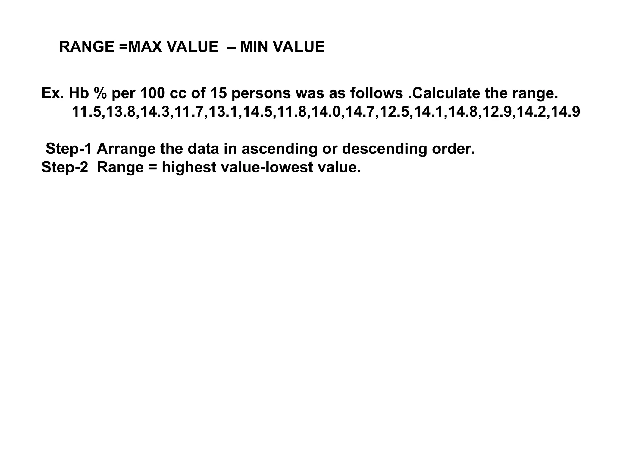
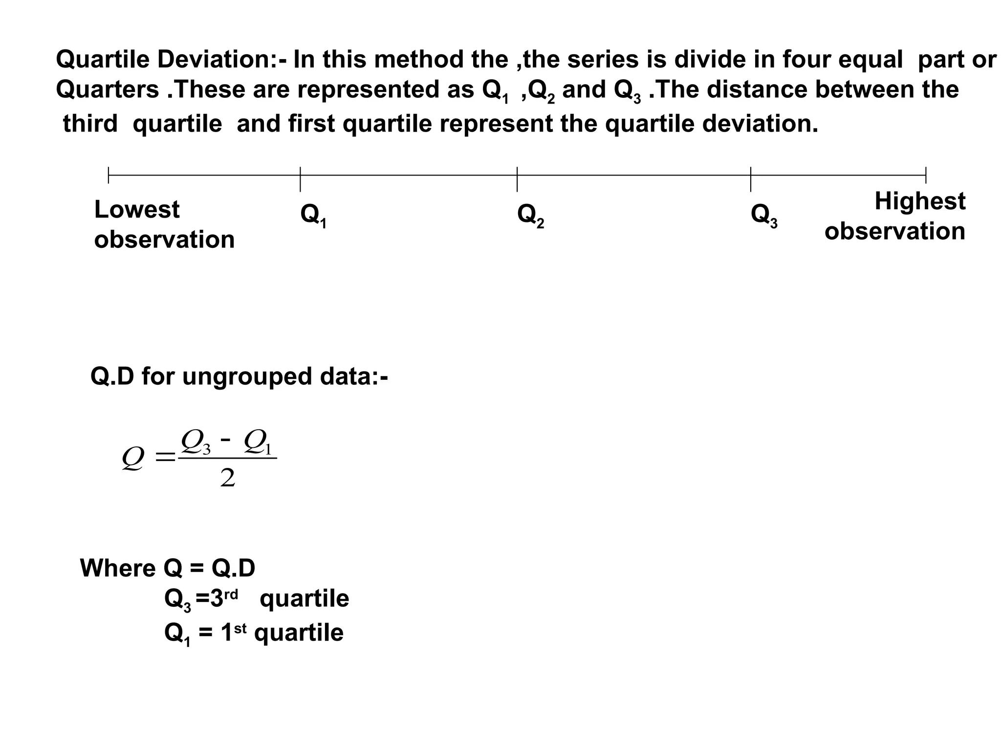
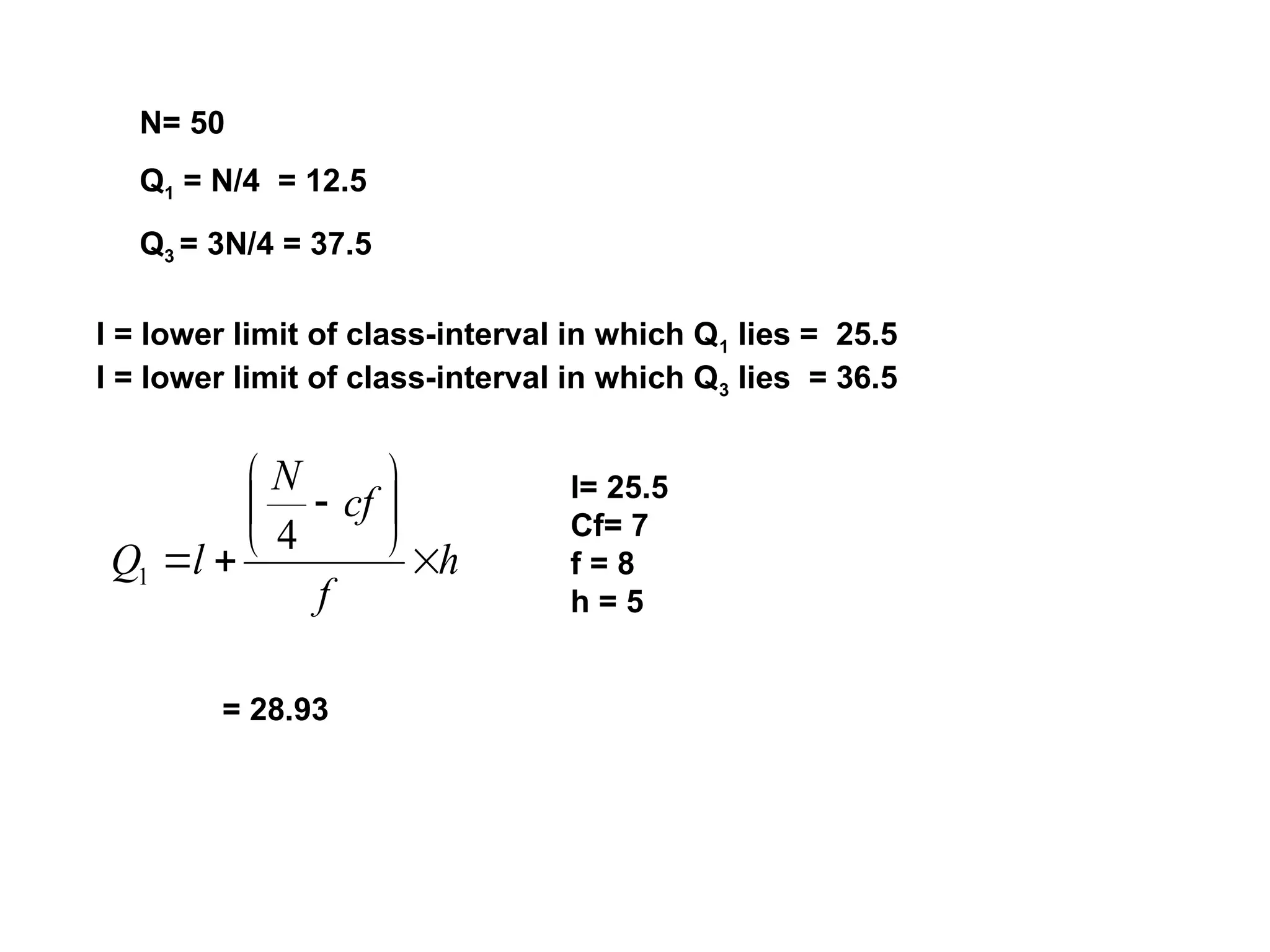
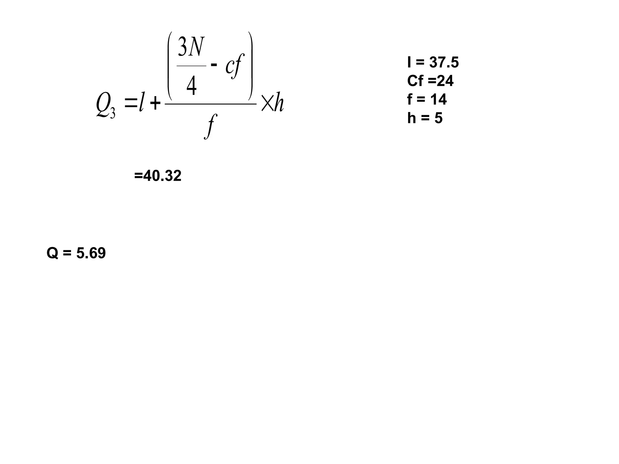
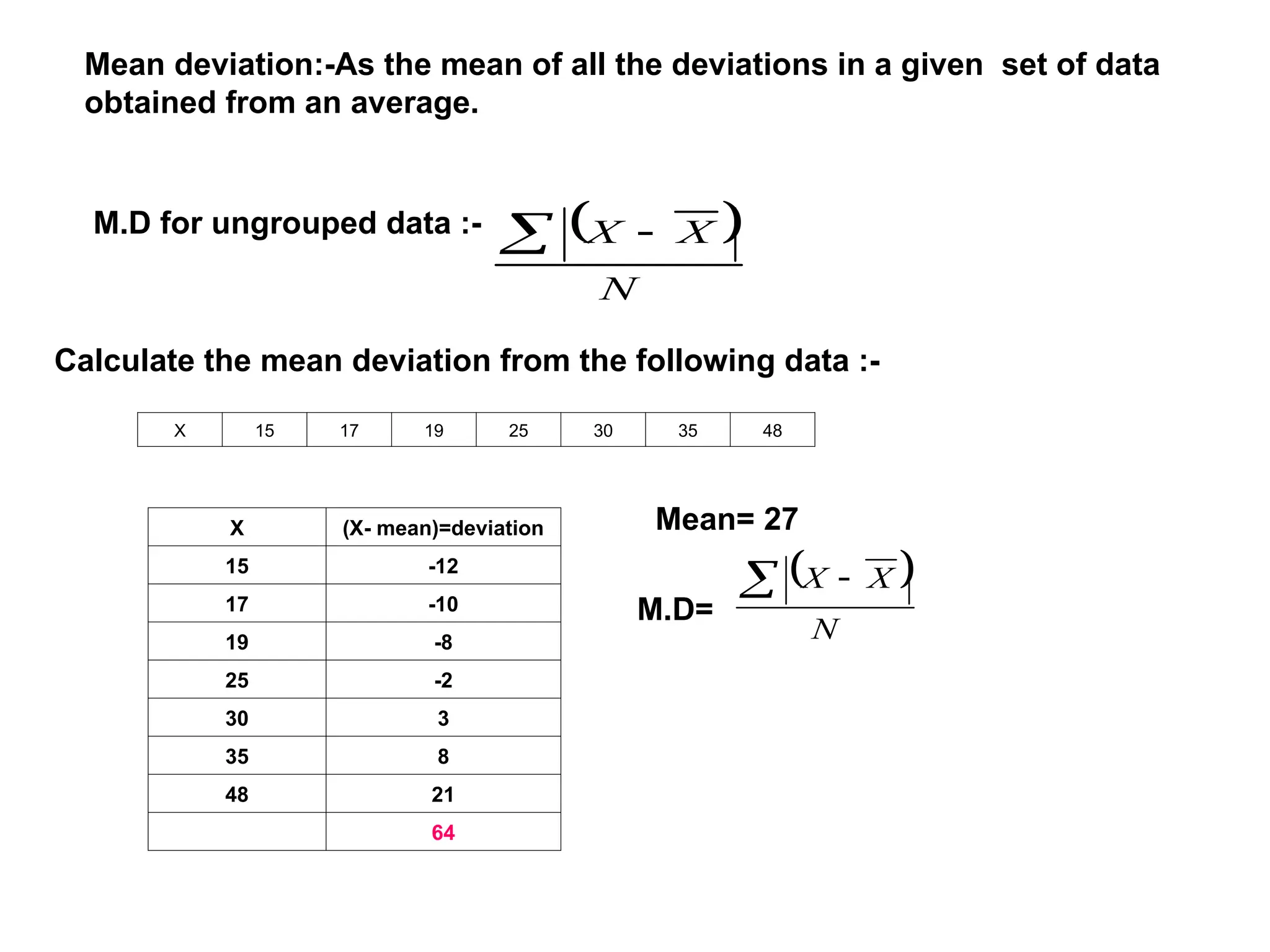
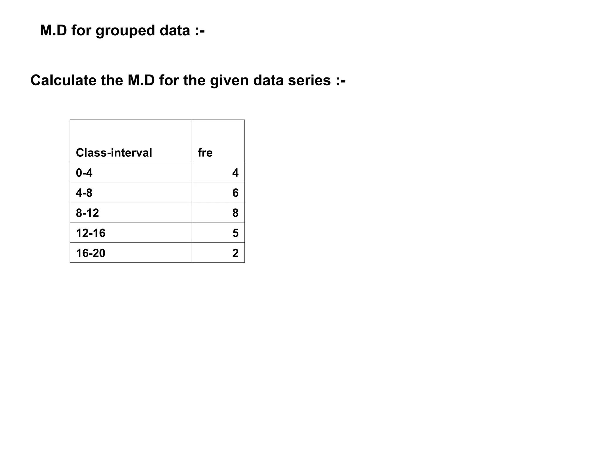
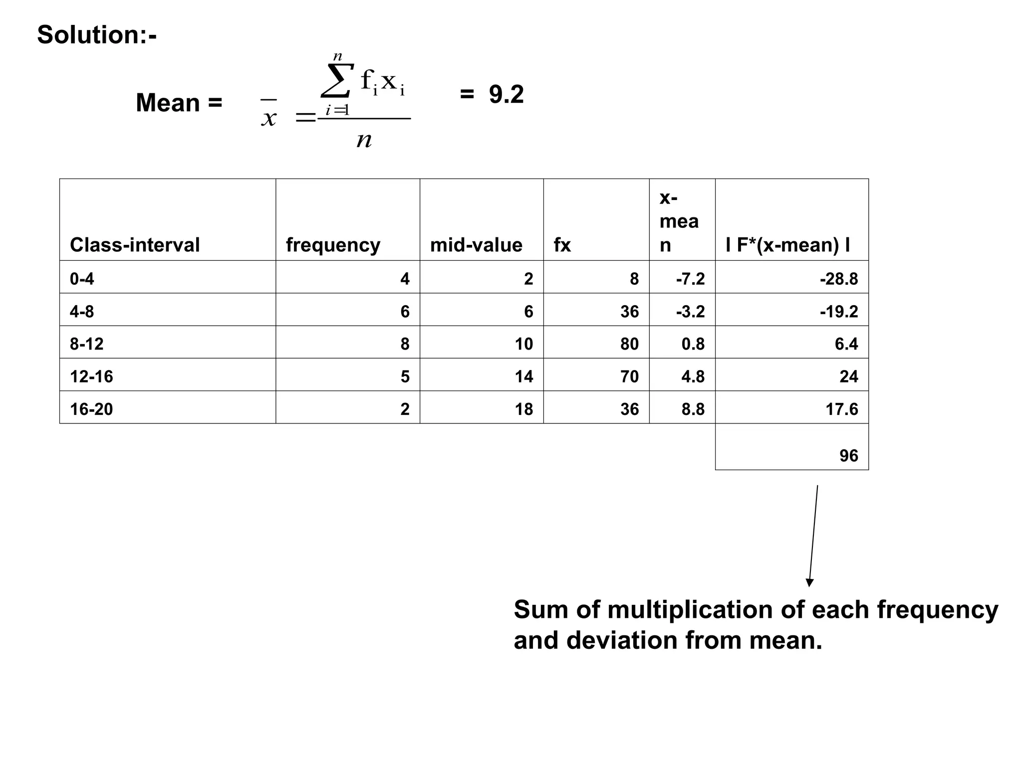
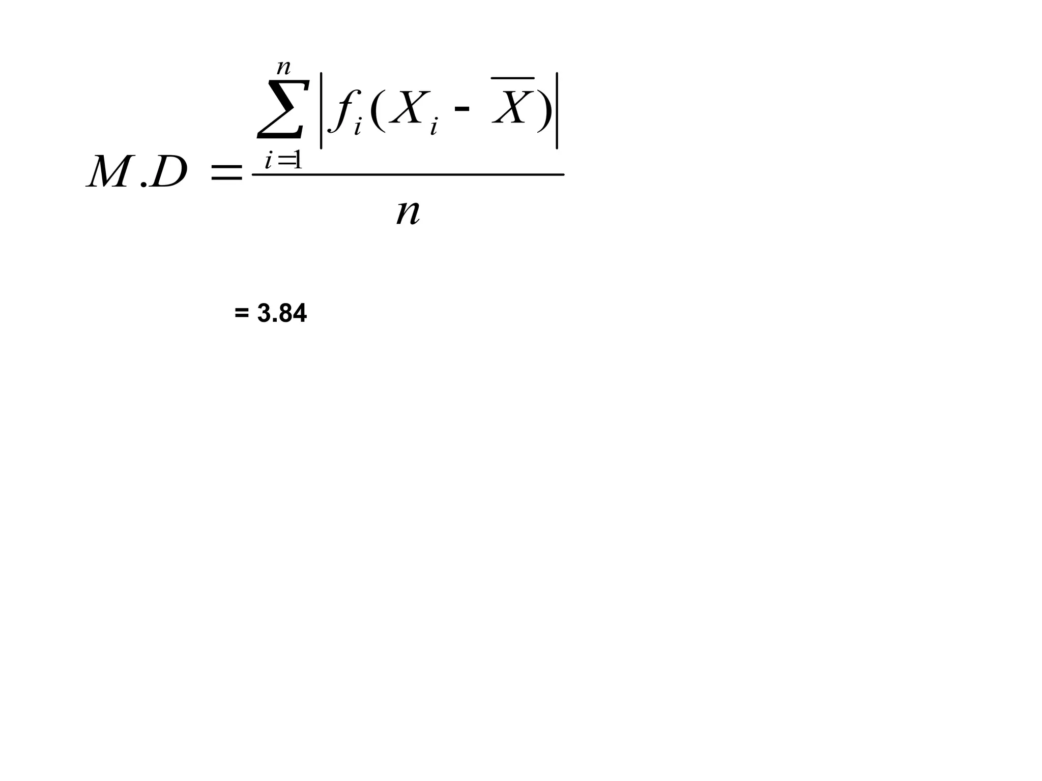
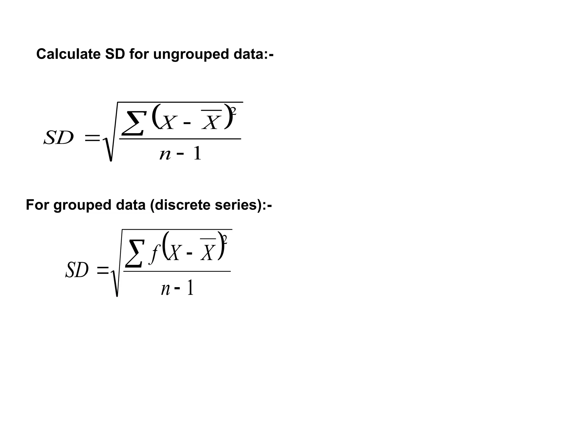
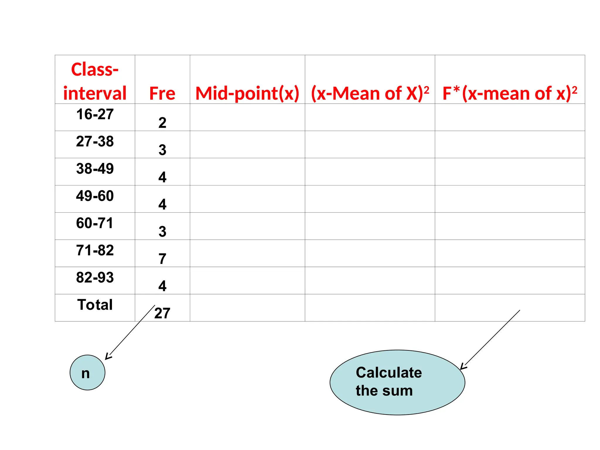
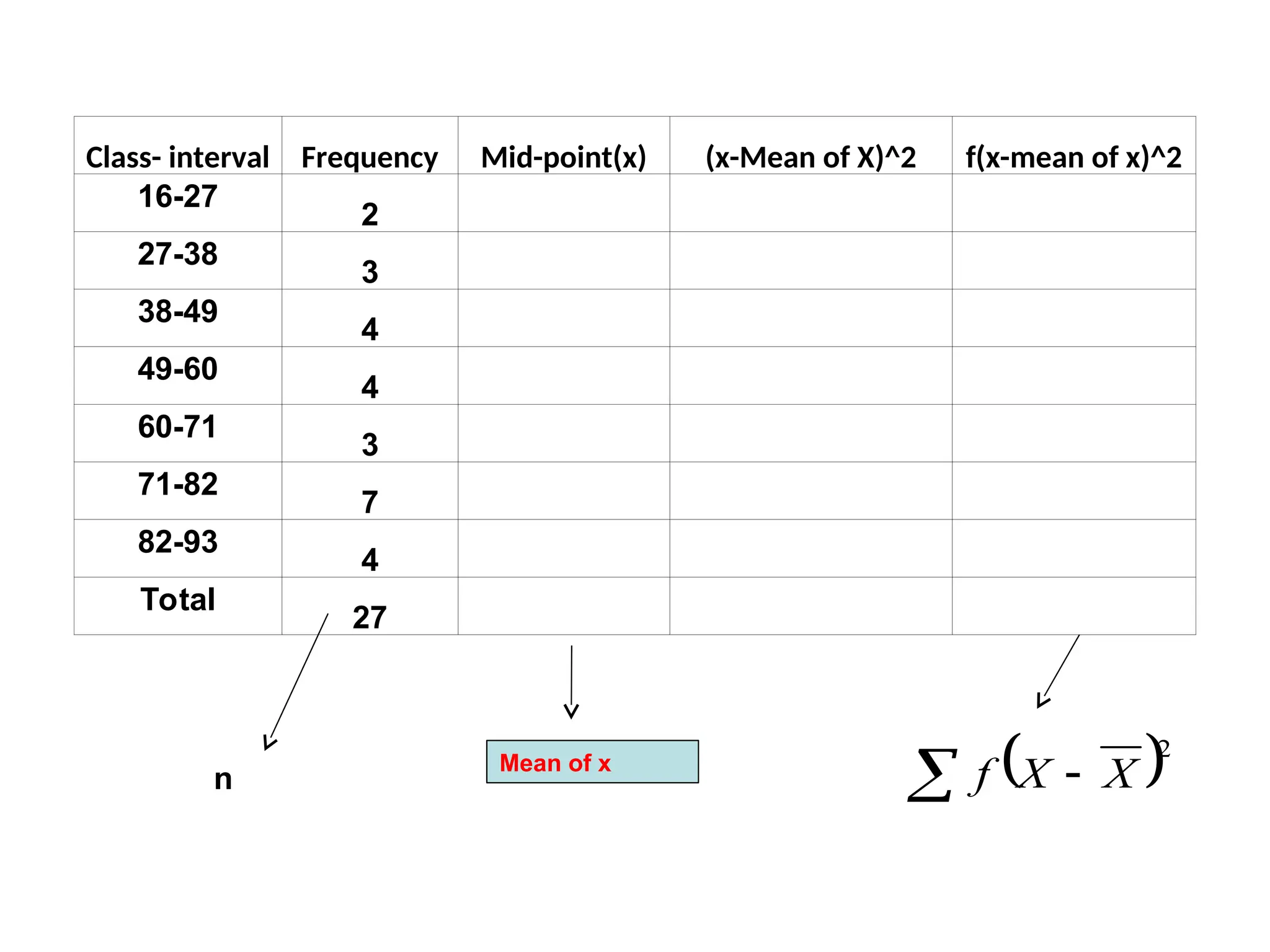
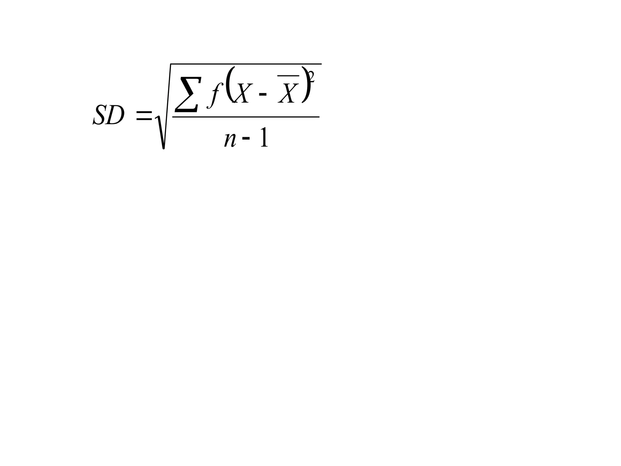
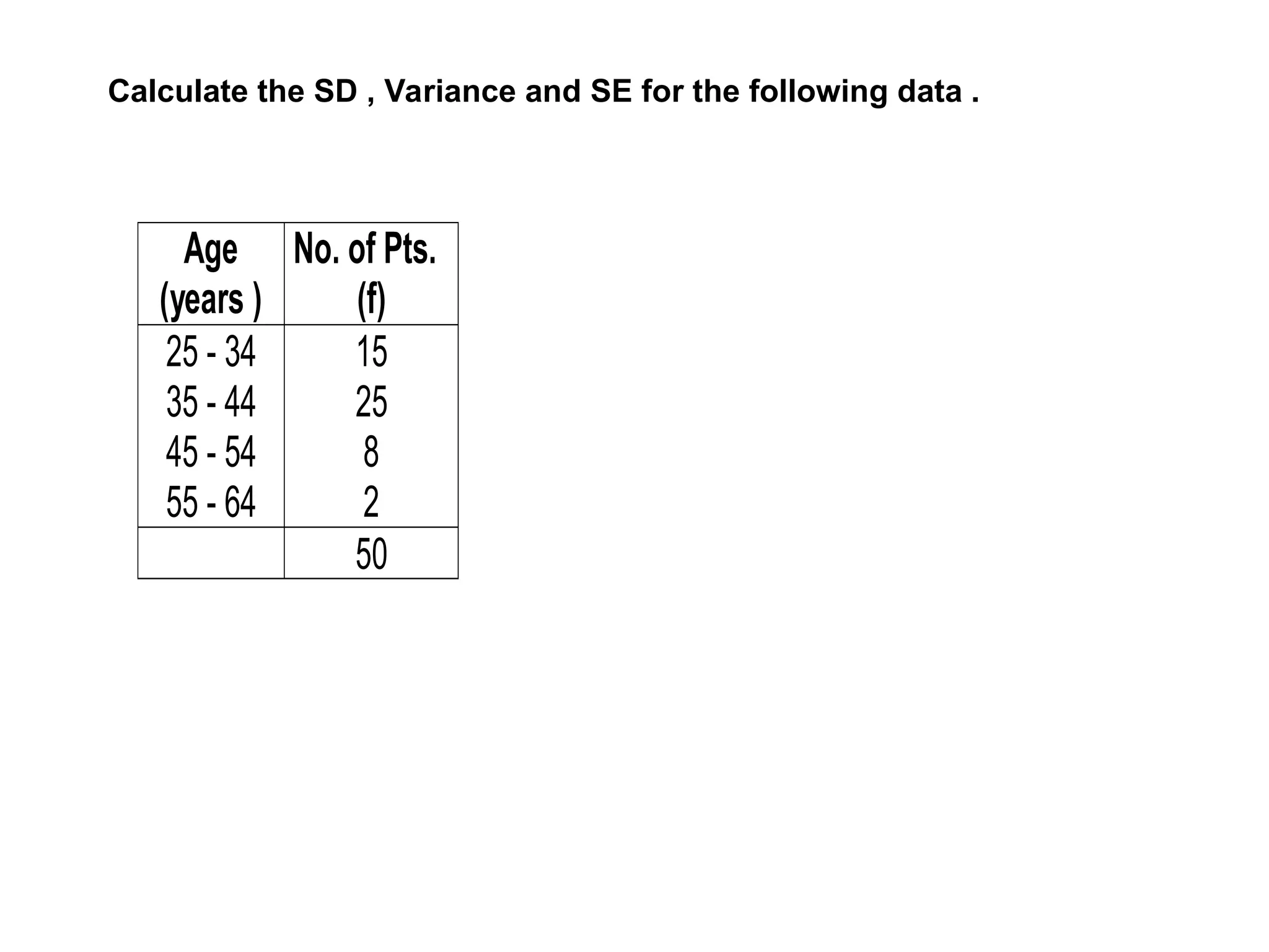
Descriptive statistics and sampling Methods ).ppt

Descriptive Statistics
& Sampling Methods
Dr. Swati Patel (M.Sc,PhD)

Descriptive Statistics
• Descriptive Statistics can be defined as a method of understanding
and presenting collected data according to type of data
i.e presentation of data with the help of table, chart and its
summarization using measure of central tendency and dispersion.
• Qualitative data can be presented as percentage or proportion
whereas, quantitative data can be presented or summarize using
measure of central tendency and Dispersion.

• Qualitative data is based on narrative
information, not numerically ‘measurable’
information (e.g., “What does age 47 feel
like?”)

Example - Details of Malaria cases are given ,this study included total
578 positive cases of malaria in SURAT in 2019,which includes patent's
Name ,Resident ,Month of case, Age, Sex, Co-morbidities present or
not ,Type of Malaria,………

• In the given study the Qualitative Variables are Residence, Sex , Month,
Co- Morbidity, Type of Malaria , Whereas Age is quantitative data.
• Sex and Residence is Binary or Dichotomous variable , whereas Months
and Type of Malaria is Categorical .
• Qualitative variables can be represented as percentage or proportion.

Out put( Presentation of data) of the given data of Malaria is as
Months a %
June 134 23%
July 111 19%
August 123 21%
Sept 53 9%
Oct 39 7%
NOV 101 17%
Dec 17 3%
Table.1 Month wise details of Malaria cases
Table -.2 Gender wise distribution of malaria cases
Sex Numbers %
Male 334 58%
Female 244 42%
Here months are qualitative (categorical data) –graphically it can be
represented as either simple bar chart or pie chart
* The given table is known as frequency table
Sex is qualitative (binary data) – graphically which
can be represented as either simple bar chart or pie chart
Similarly , we can prepare frequency table for other qualitative variables

Table :-3
Sex
Type of Malaria
Falsi Vivax Mixe Total
Male 122 114 98 334
Female 104 89 51 244
Total 226 203 149 578
Details of Type of Malaria and Sex
•The given table is known as cross table, u can make it when u have two
Qualitative variable either two ordinal , nominal or Binary
* When we have more than two qualitative data (i.e here type of malaria
and sex) - Graphically it can be represented by Multiple Bar graph or
subdivided bar graph

Distribution of malaria cases month wise
% wise presentation
Number wise presentation

Details of Type of Malaria and Sex
When we have two qualitative
variables( i.e type of malaria
and sex ) wecan use either
multiple bar diagram or
subdivided bar diagram
Multiple bar Diagram
Subdivided bar diagram

We can also prepared the graphs of previous slide like this also,

Quantitative Data
Presentation
OR
Summarization

There are two measures to summarize
the quantitative data
•Measure of Central Tendency (Mean , Median , Mode)
•Measure of Dispersion( Range, Inter Quartile Range, Standard Deviation)

MEASURE OF CENTRAL TENDANCY
MEAN
MEDIAN MODE
The average of the data
The middle value of the data most commonly occurring value

Objectives:
•Students should know which of the measures of
central tendency(mode, median, mean) are
appropriate for the different types of variables.
•Students should be able to determine the mode,
median, or mean from data presented in a table or
graph.

Relation in between Measure of central tendency

MEAN
UNGROUPED DATA GROUPED DATA
MEAN =
n
x
n
i


 1
i
x
n
x
n
i


 1
i
ix
f
MEAN =
ns
observatio
of
no.
total
ns
observatio
of
Sum

Ungrouped Data:-
Raw data or only the information regarding the Quantitative variable (i.e.
weight, height, BMI , Age, ……….) is ungrouped data.
Birth weight of new born are :
3.3kg, 3.4kg, 3.3kg,3.8kg,2.7kg,4.1kg,3.4kg,3.9kg,5.1kg,3.3kg,…………………

Grouped Data:-
The raw data is categorized in to various groups after collection of data ,and
has been organized in frequency distribution (i.e Specific variable and its
frequency)….
Day of
confinement
No of
patients
6 5
7 4
8 4
9 3
10 2
Age of
persons
at death
No. died
(f)
0-5 100
5-10 40
10-15 20
15-20 25
20-25 20
25-30 23
30-35 12
35-40 15
Discrete Grouped data
Continuous Grouped data

Duration of sickness (in days) in 10 patients is given:-
9, 7, 8 ,10 ,73 ,5 ,6 ,8 ,9 , 8
Mean = 14.3
Median = 8 days
Example of Ungrouped Data

Calculation of Mean for
Ungrouped and Grouped
Data

•Birth weight of new born :
3.3kg,6.1kg, 5.8kg,3.8kg,2.7kg,4.1kg,3.4kg,3.9kg,5.1kg,3kg.
n
x
n
i


 1
i
x
=41.2/10
=4.12 kg
•Tuberculin test reaction of 10 boys is arranged in ascending order being measured
In millimeters. Find the mean size of reaction.
3,5,7,7,8,8,9,10,11,12
Mean = 3+5+7+7+8+8+9+10+11+12/10
= 80/10
= 8 mm
Example of Ungrouped Data

For Grouped data(Discrete)
Find mean days of confinement after delivery in the following series:-
Day of
confinement
No. of
patients
6 5
7 4
8 4
9 3
10 2
Solution:-
Day of
confinement
(x)
No. of
patients
(f) X*f
6 5 30
7 4 28
8 4 32
9 3 27
10 2 20

n
x
n
i


 1
i
i x
f
=137/18
=7.61
* Find the mean age at the death in years in the following series:-
Age of
persons
at death
No. died
(f)
0-5 100
5-10 40
10-15 20
15-20 25
20-25 20
25-30 23
30-35 12
35-40 15

Age of persons
at death
No. died
(f) Mid-pint(x)
0-5 100
5-10 40
10-15 20
15-20 25
20-25 20
25-30 23
30-35 12
35-40 15
2
limit
lower
limit
Upper 
0 - 5
Upper limit
Lower limit
* When you have continuous grouped data very first step is to check the
class-inter , is it continues or not .(discontinuous class interval should
convert discontinuous to continuous class interval( + 0.5 to upper limit and
- 0.5 to lower limit)

Age of
persons
at death
No. died
(f)
mid point
(x) fx
0-5 100 2.5 250
5-10 40 7.5 300
10-15 20 12.5 250
15-20 25 17.5 437.5
20-25 20 22.5 450
25-30 23 27.5 632.5
30-35 12 32.5 390
35-40 15 37.5 562.5
255 3272.5
n
x
n
i


 1
i
i x
f
= 12.83333
Sum
n
fi 



n
i 1
i
ix
f

Median
The middle value in a set of data. Exactly half of the values lie below it,
and half lie above it.
The median can be used as a measure of central tendency for
ordinal or quantitative variables.
Perceptions of Importance of Flu
Vaccination for Pregnant Women
Visiting Prenatal Clinic #, (%)
Flu Vaccination:
Not at all important 40 (10%)
Somewhat important 80 (20%)
Very important 280 (70%)
Total 400 (100%)
There are 400 observations: the median is the 200th
-201st
observation,
which falls in the “Very important” category

For ungrouped data:-
Step-1 Arranged data in ascending or descending order.
Step:-2 If total no. of observations ‘n’ is even then used the following formula for
median= arithmetic mean of two middle observations.
Step:-3 If total no. of observations ‘n’ is odd then used the following formula for
median
.
2
1
n
observatio
th
n 


The number of patients that visited a doctor for consultation for 10 consecutive days
is arranged in an increasing order in the following table .Find out median number of
the patients that visited the doctor per day.
8,10,12,14,16,18,19,20,22,25.
n = 10
Arithmetic mean of 10 observations = 10/2 = 5 th observation
Arithmetic mean of 10 observations+1 =6 th observation
Median = 5th
observation + 6th
observation / 2
= 16+18/2
= 17
Calculate the median for the following series :-
2,3,5,1,4,5,8
1,2,3,4,5,5,8.
Median .
2
1
n
observatio
th
n 


Median:-
f
h
c
n
l








2
l = lower limit of class interval where the median occurs
f = Frequency of the class where median occurs
h = Width of the median class
C= Cumulative frequency of the class preceding the median class
Formula for continuous grouped data

For grouped Data:-
Class interval Frequency
5-9 2
10-14 11
15-19 26
20-24 17
25-29 8
30-34 6
35-39 3
40-44 2
45-49 1
Calculate the median for the following data series:-
In the given example the class interval is Discontinuous …..
Convert it in to discontinuous to continuous

Solution:-
Class
interval Frequency
cumulative
frequency
5-9 4.5-9.5 2 2
10-14 9.5-14.5 11 13
15-19 14.5-19.5 26 39
20-24 19.5-24.5 17 56
25-29 24.5-29.5 8 64
30-34 29.5-34.5 6 70
35-39 34.5-39.5 3 73
40-44 39.5-44.5 2 75
45-49 44.5-49.5 1 76
n=76
n/2= 38
l = 14.5
h = 5
f = 26
C = 13
f
h
c
n
l
Median









2 =19.31
f
cf

The mode can be obtained for any type of
variable, whether nominal, ordinal, or quantitative
(continuous or discrete).
However, the mode is the only measure of central
tendency that can used for nominal data.
Mode

Mode for ungrouped data:-
2,2,3,4,6,7,4,4,4,4,8,9,0 mode is 4
10,10,3,3,4,2,1,6,7 mode is 10 and 3
10,34,23,12,11,3,4 no mode
-In some cases ,for extraneous reasons, the interest is to identify a value
which is most common.
-Consider incubation period of measles. Perhaps ,to be able to prevent
disease in highest number of cases, it is desirable that the representative
value is estimated by the most common period of incubation .Then in this
case mode will be appropriate measure of central tendency.

Example: the mode for a nominal variable
Chief complaints of a sample of patients presenting to the Emergency Department (n=614) in
November, 2008
Chief Complaints Frequency Percent
Chest Pain 183 29.8%
Trauma/Accident 137 22.3%
Belly Pain 98 16.0%
Childbirth 44 7.2%
Dyspnea 41 6.7%
Fever 39 6.3%
Other 72 11.7%
Total 614 100.0%
The mode is “Chest Pain

Mode:- c
f
f
f
f
f
l
m
m












)
(
2
)
(
2
1
1
l = lower limit of the class where mode occurs
fm= maximum frequency of the class interval observed
f1 = frequency of the class preceding to modal class
f2 = frequency of the class interval succeeding to modal class
C= class- interval
Formula for continuous grouped data

For grouped data
Calculate the mode for the following frequency distribution:-
IQ Range Frequency
90-100 11
100-110 27
110-120 36
120-130 38
130-140 43
140-150 28
150-160 16
160-170 1
fm
f1
f2

Modal class by inspection is 130-140
fm= 43
f1= 38
f2= 28
C=10
l = 130
c
f
f
f
f
f
l
m
m












)
(
2
)
(
2
1
1
=130.6579

The most important factor to consider is:
the level of measurement or type of variable
Nominal variables: the mode is the only appropriate measure of
central tendency.
Ordinal variables: both the mode and median are used.
Quantitative variables: mode, median, and mean can all be used.
Mean is usually the measure of choice because it is a unique
value, it uses all values in the data set, and it can be used in
subsequent analyses. However, the mean is subject to extreme
(high or low) values (outliers). If the data set contains extreme
values, calculate median.

Measure of Dispersion(Variation)

MEASURES OF VARIATION
RANGE
QUARTILE
DEVIATION
MEAN
DEVIATION
STANDARD
DEVIATION
Coefficient
of
variation

RANGE =MAX VALUE – MIN VALUE
Ex. Hb % per 100 cc of 15 persons was as follows .Calculate the range.
11.5,13.8,14.3,11.7,13.1,14.5,11.8,14.0,14.7,12.5,14.1,14.8,12.9,14.2,14.9
Step-1 Arrange the data in ascending or descending order.
Step-2 Range = highest value-lowest value.

Quartile Deviation:- In this method the ,the series is divide in four equal part or
Quarters .These are represented as Q1 ,Q2 and Q3 .The distance between the
third quartile and first quartile represent the quartile deviation.
Q1 Q2 Q3
Lowest
observation
Highest
observation
Q.D for ungrouped data:-
2
1
3 Q
Q
Q


Where Q = Q.D
Q3 =3rd
quartile
Q1 = 1st
quartile

Q.D for ungrouped data:-
Find the Q.D for the following data series:-
8,12,13,9,11,17,23,25,20,21,27.
Step:-1 Arrange the data in ascending order
8,9,11,12,13,17,20,21,23,25,27.
Step-2 Find out first and third quartile
  value
N
Q
value
N
Q
th
th
4
1
3
&
4
1
3
1







 

Step-4 Q1 = 11+1/4 = 3 rd value = 11
Q3= 3(11+1)/4 = 9 th value = 23
Step- 5 2
1
3 Q
Q
Q


= 23-11/2 = 6

Q.D for grouped data (Discrete series) :-
Step-1 Calculate the frequency and c.f from the data given.
Step:-2 Calculate the lower and upper quartile heights by using the formula
 
4
1
3
&
4
1
3
1







 

N
Q
N
Q
Step:-3 Apply the value of Q1 and Q3 in the formula
2
1
3 Q
Q
Q



Eg) Frequency distribution of height in cm of 387 students in a school is given
in the table below .Find the inter quartile range and Q.D of height distribution.
Height in cmc No. of students
150 28
152 40
154 52
156 100
158 60
160 48
162 32
164 20
166 7

Height in cmc
No. of
students c.f
150 28 28
152 40 68
154 52 120
156 100 220
158 60 280
160 48 328
162 32 360
164 20 380
166 7 387
Step:-1 Find the C.F
Step:-2
 
4
1
3
&
4
1
3
1







 

N
Q
N
Q
Q1 of the data = 97th
students and Q3 of the data = 291st
students
97 student is included in the 3rd
group having height 154 cm.
291 student is including in the 6th
group having height 160 cm
Q1 = 154, Q3= 160 .

Inter Quartile range = (Q1-Q3) = 154- 160cm
Q.D = 3

Q.D for the grouped data ( continuous series):-
h
f
cf
N
l
Q
h
f
cf
N
l
Q




















4
3
4
3
1
Apply the value of Q1 and Q3 in the formula
2
1
3 Q
Q
Q



Eg. Water percentage in the body of species of fish and their
frequency is given in the table below. Calculate the Q.D.
sr.no Class interval fre
1 16-20 4
2 21-25 3
3 26-30 8
4 31-35 9
5 36-40 14
6 41-45 3
7 46-50 3
8 51-55 2
9 56-60 2
10 61-65 2

sr.no
Class
interval fre c.f
1 16-20 15.5-20.5 4 4
2 21-25 20.5-25.5 3 7
3 26-30 25.5-30.5 8 15 Q1
4 31-35 30.5-35.5 9 24
5 36-40 35.5-40.5 14 38 Q3
6 41-45 40.5-45.5 3 41
7 46-50 45.5-50.5 3 44
8 51-55 50.5-55.5 2 46
9 56-60 55.5-60.5 2 48
10 61-65 60.5-65.5 2 50

N= 50
Q1 = N/4 = 12.5
Q3 = 3N/4 = 37.5
l = lower limit of class-interval in which Q1 lies = 25.5
l = lower limit of class-interval in which Q3 lies = 36.5
h
f
cf
N
l
Q 









4
1
l= 25.5
Cf= 7
f = 8
h = 5
= 28.93

h
f
cf
N
l
Q 









4
3
3
l = 37.5
Cf =24
f = 14
h = 5
=40.32
Q = 5.69

Mean deviation:-As the mean of all the deviations in a given set of data
obtained from an average.
M.D for ungrouped data :-  
N
X
X
 
Calculate the mean deviation from the following data :-
X 15 17 19 25 30 35 48
X (X- mean)=deviation
15 -12
17 -10
19 -8
25 -2
30 3
35 8
48 21
64
M.D=
 
N
X
X
 
Mean= 27

M.D for grouped data :-
Calculate the M.D for the given data series :-
Class-interval fre
0-4 4
4-8 6
8-12 8
12-16 5
16-20 2

Solution:-
Class-interval frequency mid-value fx
x-
mea
n l F*(x-mean) l
0-4 4 2 8 -7.2 -28.8
4-8 6 6 36 -3.2 -19.2
8-12 8 10 80 0.8 6.4
12-16 5 14 70 4.8 24
16-20 2 18 36 8.8 17.6
96
Mean =
n
x
n
i


 1
i
i x
f
= 9.2
Sum of multiplication of each frequency
and deviation from mean.

n
X
X
f
D
M
n
i
i
i



 1
)
(
.
= 3.84

Standard deviation:- S.D is an important measure of dispersion.
•A large S.D shows that the measurements of the frequency distribution are
widely spread out from the mean..
eg. 10 mm in case of BP.
• A small S.D shows that the measurements of the frequency distribution are
closely spread in the neighborhood of mean.
eg 2cm in case of height.
• SD helps us to predict how far a given value is always from mean.
Use of SD:-
When populations are combined or when samples are combined their
SD pooled after appropriate reasoning.
Eg. Comparison of Surgical treatment for cancer lung from two studies
may require knowledge of respective SD which are subsequently
pooled

Calculate SD for ungrouped data:-
 
1
2




n
X
X
SD
For grouped data (discrete series):-
 
1
2




n
X
X
f
SD

For grouped data (continuous):-
 
n
X
X
f
SD
 

2
OR
2
2












n
fx
n
fx
SD

Ex. Find the SD, variance and SE of the ESR ,found to be
3,4,5,4,2,4,5 and 3 in 8 normal individuals.
3
4
5
4
2
4
5
3
i
X 2
)
( X
Xi 
Step- 1 , Calculate the mean of x.
sum
n
x
n
i


 1
i
x
sum

Ex. Find the SD of the ESR ,found to be 3,4,5,4,2,4,5 and 3 in 8 normal individuals
3
4
0.0625
5 1.5625
4 0.0625
2 3.0625
4 0.0625
5 1.5625
3 0.5625
30 7.5
3.75
i
X 2
)
( X
Xi 
MEAN
sum
0.5625
 
1
2




n
X
X
SD
=
7
5
.
7
= 1.03

Class- interval Frequency
16-27 2
27-38 3
38-49 4
49-60 4
60-71 3
71-82 7
82-93 4
Total 27
Ex. Calculate the SD , Variance and SE for the following data .

Class-
interval Fre Mid-point(x) (x-Mean of X)2
F*(x-mean of x)2
16-27
2
27-38
3
38-49
4
49-60
4
60-71
3
71-82
7
82-93
4
Total
27
n Calculate
the sum

Class- interval Frequency Mid-point(x) (x-Mean of X)^2 f(x-mean of x)^2
16-27
2
27-38
3
38-49
4
49-60
4
60-71
3
71-82
7
82-93
4
Total
27
n
Mean of x
 
 
2
X
X
f

 
1
2




n
X
X
f
SD

Age
(years )
No. of Pts.
(f)
25 - 34
35 - 44
45 - 54
55 - 64
15
25
8
2
50
Calculate the SD , Variance and SE for the following data .

Coefficient of variation:-
it is one of the useful terms which is used to compare the variability
of two diverse population with different units of Measure like height
by weight , BP by blood cell diameters.
100


mean
SD
CV
It express the size of SD in relation to the size of mean and further converted to
percentage.
Ex. In a Series of boys ,the mean systolic BP was 120 and SD was 10 .In the
same series mean height and SD were 160 cm and 5 cm ,respectively. Find
which character show greater variation?
CV of BP = 8.3%
CV of height = 3.1%
Thus , BP found to be a more character than height, 8.3/3.1 =2.7times.

Ex)The study was conducted to know the effect of Vit.D3 supplementation
in DM type-2 patients ,which includes age, sex,vit D3 pre &post,HbA1c
pre& post, FBS pre and post ……….

This study includes qualitative and quantitative both variables, where
gender is only qualitative (binary) variable reaming all others are
quantitative, Which can be represented by Mean and Standard deviation.

Study Variables N Mean SD
Age 78 56 9.152221
Vit D3 level 78 27.94987 13.53687
HbA1C level 78 7.964156 1.804317
FBS__pre 78 140.7143 42.39472
PPBS_pre 78 210.4935 74.03726
Vit D3_post 78 34.62117 11.79473
HbA1C_post 78 7.350649 1.616659
Quantitative Variables which represented by Mean and SD
Note: when some extreme values present in the given data(quantitative) ,which can be
represented as MEDIAN &INTERQUARTILE RANHGE instead of Mean and SD

Sampling Techniques
D ATA COLLECTION METHOD

What is Sampling?
• Sampling is a statistical procedure that is
concerned with the selection of the
individual observation; it helps us to make
statistical inferences about the population.

What is Population?
Population is an entire group of study.
+ve patients of HIV in Surat
city
Population

What is Sample?
• Sample is the part of Population.
+ve patients
of HIV in
Surat city
+ve patient of HIV
under taking the
treatment in SMIMER
Population
Sample

Population
Sample
Sample is subset of
population

Sample
Target population
Study population

Why sampling?
Get information about large populations
 Less costs
 Less field time
 More accuracy i.e. Can Do A Better Job of
Data Collection
 When it’s impossible to study the whole
population

Types of sampling
• Non-probability sampling
• Probability sampling

Sampling Techniques:-
Probability sampling
1)Simple random sampling
2) Systematic sampling
3) Stratified random sampling
4)Cluster sampling
5) Multistage sampling
6) Multiphase sampling

Simple random sampling
What is it?
Every individual of population has an equal chance to be
selected.
When we can apply?
When the population is Small, Homogeneous and readily available.
Eg) Patients coming to the Hospital or admitted in the ward.
SRS
Lottery
Method
Random
Number Table

Table of random numbers
6 8 4 2 5 7 9 5 4 1 2 5 6 3 2 1 4 0
5 8 2 0 3 2 1 5 4 7 8 5 9 6 2 0 2 4
3 6 2 3 3 3 2 5 4 7 8 9 1 2 0 3 2 5
9 8 5 2 6 3 0 1 7 4 2 4 5 0 3 6 8 6
…………………….

EX) Select a sample of 10 from a population of 300 female patients
attending the MCH.
---- Step 1 ) 300 is the three digit figure.
First three rows of the random table are chosen.
034 ,977 ,167 , 125 , 555 , 162 , 844 , 630 , 332 , 576 .
The number selected for the sample will be
34 , 77,167 ,125,255,162,244,32,276,
If some numbers repeated ,they can be rejected .

Systematic sampling
Population
Large ,Scattered and Homogeneous
Process of selection of sample:-
desired
Size
Sample
Population
Total
Fraction
Sampling
K 

10% of sample to be taken out of 1000 population

10
1000
%
10
1000


of
K
Step- 1 Calculate the K.
Step:- 2 Select any one number randomly (from random no. table) from 1 to 10.
Step:- 3 Supposing it is 6 .
Step :- 4 for second sample no 10+6 = 16
For third sample 16+10 =26
26+10 = 36 and so on.

Stratified Sampling
Population Large and not Homogeneous
The population first we divided in the homogeneous group
That groups or classes are called strata

Cluster sampling
Cluster Is a randomly selected group
Cluster: a group of sampling units close to each other i.e. crowding
together in the same area or neighborhood

Cluster sampling is an example of 'two-stage sampling' .
*First stage a sample of areas is chosen;
•Second stage a sample of respondents within those areas is selected.
*Population divided into clusters of homogeneous units, usually
based on geographical contiguity.
*Sampling units are groups rather than individuals.
*A sample of such clusters is then selected.
*All units from the selected clusters are studied.

Advantages :
Cuts down on the cost of preparing a sampling
frame.
This can reduce travel and other administrative
costs.
Disadvantages: sampling error is higher for a
simple random sample of same size.
Often used to evaluate vaccination coverage in
EPI

•Identification of clusters
–List all cities, towns, villages & wards of cities with their
population falling in target area under study.
–Calculate cumulative population & divide by 30, this gives
sampling interval.
–Select a random no. less than or equal to sampling interval
having same no. of digits. This forms 1st
cluster.
–Random no.+ sampling interval = population of 2nd
cluster.
–Second cluster + sampling interval = 4th
cluster.
–Last or 30th
cluster = 29th
cluster + sampling interval

• Freq c f cluster
• I 2000 2000 1
• II 3000 5000 2
• III 1500 6500
• IV 4000 10500 3
• V 5000 15500 4, 5
• VI 2500 18000 6
• VII 2000 20000 7
• VIII 3000 23000 8
• IX 3500 26500 9
• X 4500 31000 10
• XI 4000 35000 11, 12
• XII 4000 39000 13
• XIII 3500 44000 14,15
• XIV 2000 46000
• XV 3000 49000 16
• XVI 3500 52500 17
• XVII 4000 56500 18,19
• XVIII 4500 61000 20
• XIX 4000 65000 21,22
• XX 4000 69000 23
• XXI 2000 71000 24
• XXII 2000 73000
• XXIII 3000 76000 25
• XXIV 3000 79000 26
• XXV 5000 84000 27,28
• XXVI 2000 86000 29
• XXVII 1000 87000
• XXVIII 1000 88000
• XXIX 1000 89000 30
• XXX 1000 90000
• 90000/30 = 3000 sampling interval

Multi stage Sampling
Employee in large country survey
In the first stage random no. of district are chosen in all the stage
Then talukas ,
villages
Then third stage units will be houses.
All ultimate units (houses, for
instance) selected at last step are
surveyed.

MULTI PHASE SAMPLING
Part of the information collected from whole
sample & part from subsample.
In Tb survey MT in all cases – Phase I
X –Ray chest in MT +ve cases – Phase II
Sputum examination in X – Ray +ve cases -
Phase III
Survey by such procedure is less costly, less
laborious & more purposeful

Multiphase sampling:-
In Tuberculosis
Survey
First Phase Physical examination or
Manteux test
(In +ve patients )
Chest X-ray may be done in
Mantoux +ve test
Sputum may be examine in X-ray
+ve cases

Non probablity Sampling Methods
•Convenience Sampling
•Quota sampling
•Purposive sampling

•It is non probability sampling.
•Sample is selected as a matter of convenience not
bases on the probability theory .
•For example , in clinical practice , doctors might uses
patients who are available to him/her.
Convenience Sampling

Involves sampling a quota of units to be selected from
each population cell based on the judgment of the
researchers and/or decision makers
Steps
1) Divide the population into segments (referred to
as cells) based on certain control characteristics
2) Determine the quota of units for each cell (quotas
are determined by the researchers and/or decision
makers)
3) Instruct the interviewers to fill the quotas assigned
to the cells
Quota Sampling

•Purposive sampling
•If some characteristics of the population are
known as a
result of previous survey, samples are chosen
by purposive selection .
•As result ,certain features of sample selected
purposively are likely to tally with those
of population .
•Also due to scarcity of time , limitation of
investigators and scarcity of funds.

Sampling and Non-Sampling Errors…
Two major types of error can arise when a sample of
observations is taken from a population:
sampling error and no sampling error.
Sampling error refers to differences between the sample
and the population that exist only because of the
observations that happened to be selected for the sample.
Random and we have no control over.
Non sampling errors are more serious and are due to
mistakes made in the acquisition of data or due to the
sample observations being selected improperly. Most likely
caused be poor planning, sloppy work, act of the Goddess
of Statistics, etc.

Sampling Error…
Sampling error refers to differences between
the sample and the population that exist only
because of the observations that happened to
be selected for the sample.
Increasing the sample size will reduce this type
of error.

Non sampling errors are more serious and are due to
mistakes made in the acquisition of data or due to the
sample observations being selected improperly.
Three types of non sampling errors:
Errors in data acquisition,
Nonresponse errors, and
Selection bias.
Note: increasing the sample size will not reduce this
type of error.
Non sampling Error…

5.104
Errors in data acquisition…
• …arises from the recording of incorrect
responses, due to:
• — incorrect measurements being taken because of faulty
equipment,
• — mistakes made during transcription from primary sources,
• — inaccurate recording of data due to misinterpretation of
terms, or
• — inaccurate responses to questions concerning sensitive
issues.

5.105
Nonresponse Error…
• …refers to error (or bias) introduced when
responses are not obtained from some members
of the sample, i.e. the sample observations that
are collected may not be representative of the
target population.
• As mentioned earlier, the Response Rate (i.e. the
proportion of all people selected who complete the
survey) is a key survey parameter and helps in the
understanding in the validity of the survey and
sources of nonresponse error.

5.106
Selection Bias…
• …occurs when the sampling plan is such
that some members of the target
population cannot possibly be selected for
inclusion in the sample.

1) What is the median of the following set of scores?
18, 6, 12, 10, 14
2) We consider observations reporting the eye color of a group of 15
people: Brown, Brown, Blue, Brown, Green, Gray, Blue, Blue, Green,
Brown, Gray, Brown, Brown, Blue, Green.
1.Construct a frequency table.
2. Draw the associated bar graph.
3) Ten patients at a doctor’s surgery wait for the following lengths of
times to see their doctor. 5 mins ,17 mins, 8 mins ,2 mins, 55 mins, 9
mins, 22 mins ,11mins, 16 ,5 mins .What are the mean, median and mode
for these data? What measure of central tendency would you use here?
4) Calculate the mean and standard deviation of the following set of data.
Birth weight of ten babies (in kilograms) 2.977 3.155 3.920 3.412 4.236
2.593 3.270 3.813 4.042 3.387

5. In a survey of sleep apnea scores among 10
people, the highest sample of 58 was entered by
mistake as 85. This will affect the result as
1.Increased mean, increased median
2.Increased mean, no change in median
3.Non-change in mean, increase median
4.Increased mean, decreased median

1.Histogram
2.Line diagram
3.Box and Whisker plot
4.Kaplan Meyer plot
Identify the diagram shown

Likert scale is?
1.Ordinal scale
2.Nominal scale
3.Variance scale
4.Categorical scale

The individual in a village population is
arranged alphabetically and every
8th
person is selected for the study. The type
of study is
1.Simple random sampling
2.Stratified random sampling
3.Systemic random sampling

A study done on a group of patients showed a coefficient of
variance of BP and serum creatinine to be 20% & 15%
respectively. Inference is that
1.Variation of BP is more than in serum creatinine
2.Variation in serum creatinine is more than in BP
3.The standard deviation of BP is more than of creatinine
4.The standard deviation of creatinine is more than of BP

Which is not a measure Of dispersion?
1.Mean deviation
2.Standard deviation
3.Mode
4.Range

Scatter diagram represents
1.Frequency of occurrence
2.Trend over time
3.Correlation / Association
4.None of the above

Research selected all possible samples from a
population and plotted their means on a line graph.
This distribution is called as
1.Sample distribution
2.Sampling distribution
3.Population distribution
4.Parametric distribution

Measuring relative variation between two different units is done by
1.variance
2.coefficient of variation
3.standard deviation
4.range

The median weight of 100 children was 12 kg and it formed a
normal distribution. The standard deviation was 3. Calculate the
percentage of coefficient of variation.
1.25%
2.35%
3.45%
4.55%

Stratified sampling is ideal for
1.Heterogenous data
2.Homogenous data
3.Both
4.None

Which of the following is/are non-random sampling
methods-
a) Quota sampling
b) Stratified random sampling
c) Convenience Sampling
d) Cluster Sampling
1.ab
2.bc
3.ac
4.cd

10.True statements with regard to sampling-
a) Snowball sampling is used for a hidden population
b) More sample in systemic random sampling
c) In stratified random sampling, the population is divided
into strata
d) Cluster sampling is less cost-effective
1.ab
2.bc
3.ac
4.cd

11.The upper and lower limit of standard errors
within which a parameter value is expected to lie
are called as
1.confidence interval
2.confidence limit
3.precision levels
4.accuracy limit
Ans (confidence limit)

12.Evidence-based medicine, which of the following is not useful –
a) Personal exposure
b) RCT
c) Case report
d) Meta-analysis
e) Systemic review
1.ab
2.bc
3.ac
4.cd
Ans (ac)

13.If mean is 230 and standard error is 10 then 95% of
confidence limit is
1.210-250
2.250-290
3.290-330
4.190-210
Ans (210-250)

17.Which one of the following is not a measure of dispersion –
1.Mean
2.Range
3.Mean deviation
4.Standard deviation
Ans (Mean)

19.In a normal curve, the area of one
standard deviation around the mean
includes which of the following
percent of values in a distribution –
1.0.486
2.0.683
3.0.954
4.0.997
Ans (0.683)

Of a set of values is that value which
occurs most frequently.
(a) Mean
(b) The Mode
(c) Median
(d) Standard deviation.

The SD is an appropriate measure of spread when centre is measured
with the
a) Mean
b) Median
c) Mode
d) None of the above

The PEFR of a group of 11 year old
girls follow a normal distribution with
mean 300 l/min and standard
deviation 20 l/min:
A. About 95% of the girls have PEFR
between 260 and 340 l/min
B. The girls have healthy lungs
C. About 5% of girls have PEFR below
260 l/min
D. All the PEFR must be less than 340
l/min
Correct answer : A. About 95% of the
girls have PEFR between 260 and 340
l/min
•95.4% of values lie within 2 SD
(standard deviation) of the mean
•Here, SD = 20 l/min
•Hence 95.4% of values lie within
300-(2*20) and 300=(2*20)
•Which translates into : About 95%
of the girls have PEFR between 260
and 340 l/min

Descriptive statistics and sampling Methods ).ppt

More Related Content

Similar to Descriptive statistics and sampling Methods ).ppt

Recently uploaded

Descriptive statistics and sampling Methods ).ppt