Download as PDF, PPTX
![[course site]
Santiago Pascual de la Puente
santi.pascual@upc.edu
PhD Candidate
Universitat Politecnica de Catalunya
Technical University of Catalonia
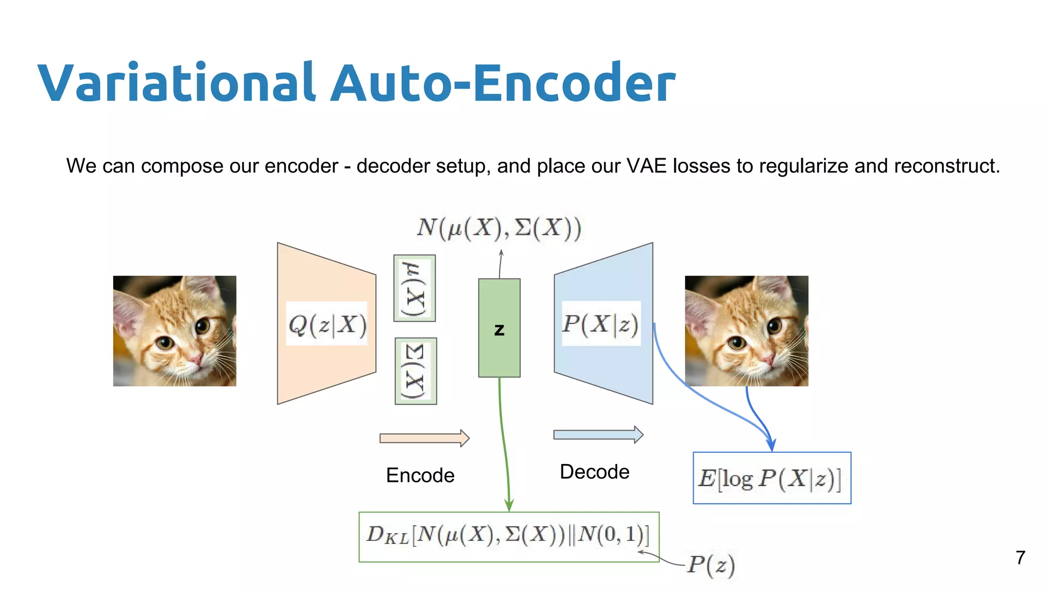
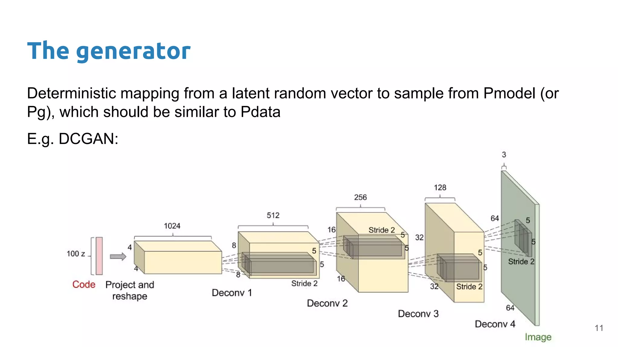
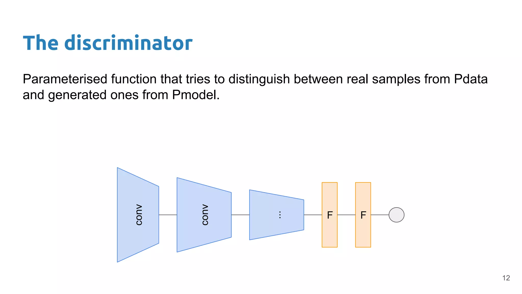
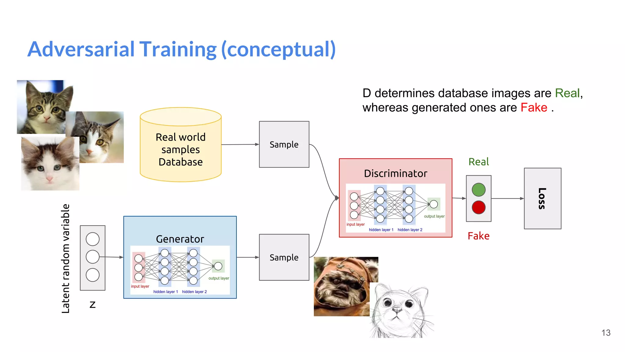
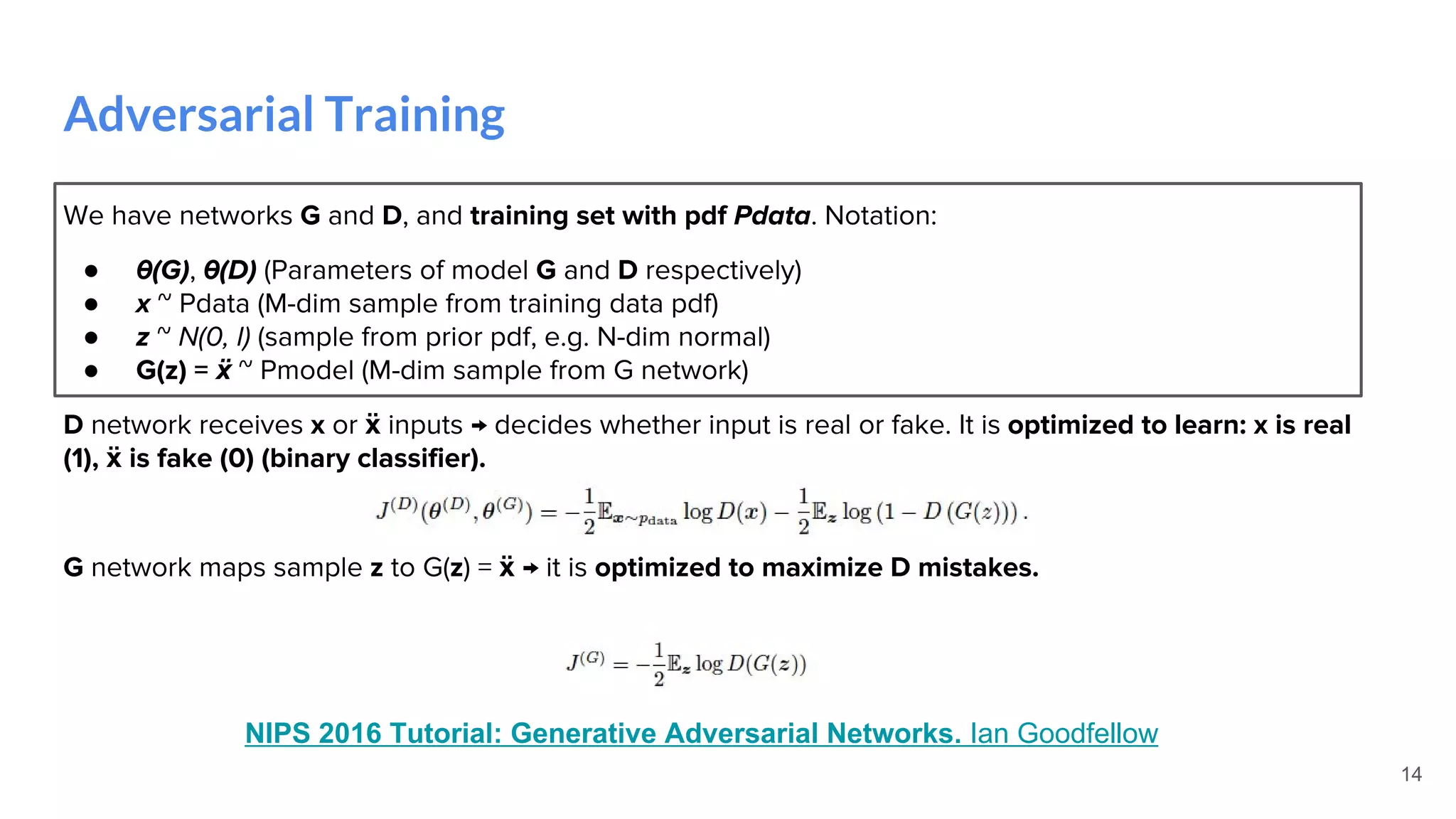
Deep Generative Models II
#DLUPC](https://image.slidesharecdn.com/dlai2017d10l1-171228154829/75/Deep-Generative-Models-II-DLAI-D10L1-2017-UPC-Deep-Learning-for-Artificial-Intelligence-1-2048.jpg)


![[course site]
Santiago Pascual de la Puente
santi.pascual@upc.edu
PhD Candidate
Universitat Politecnica de Catalunya
Technical University of Catalonia
Deep Generative Models II
#DLUPC](https://crownmelresort.com/image.slidesharecdn.com/dlai2017d10l1-171228154829/75/Deep-Generative-Models-II-DLAI-D10L1-2017-UPC-Deep-Learning-for-Artificial-Intelligence-1-2048.jpg)


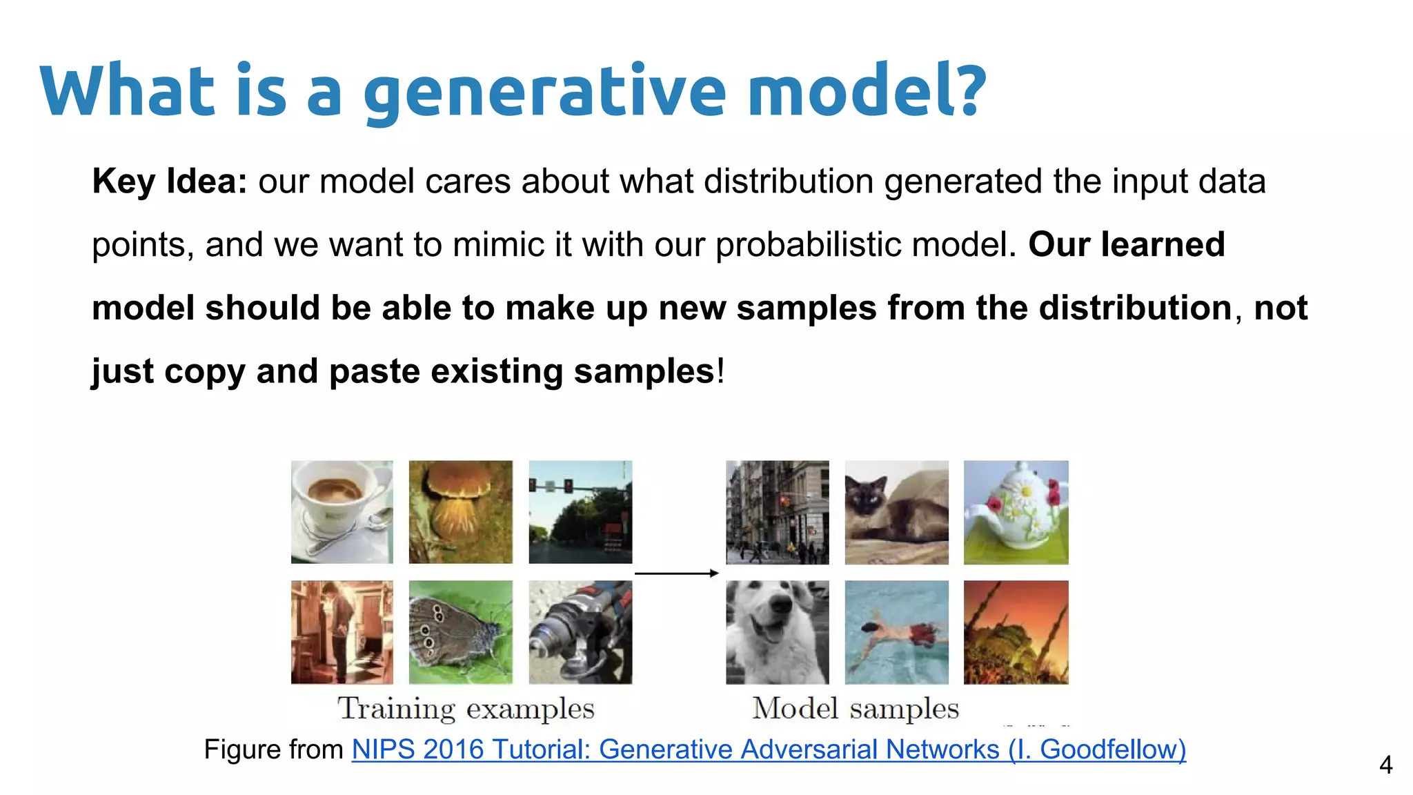
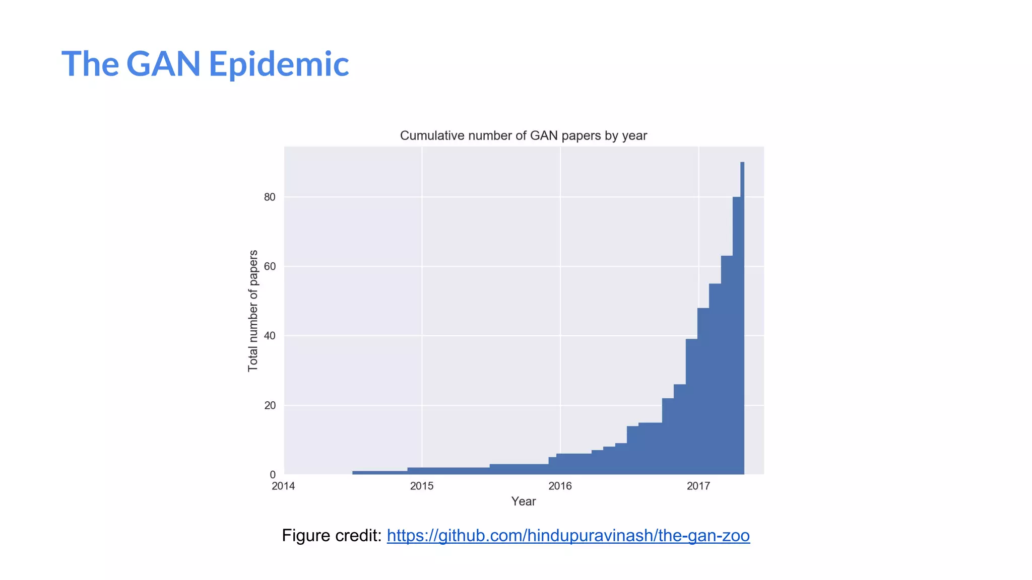
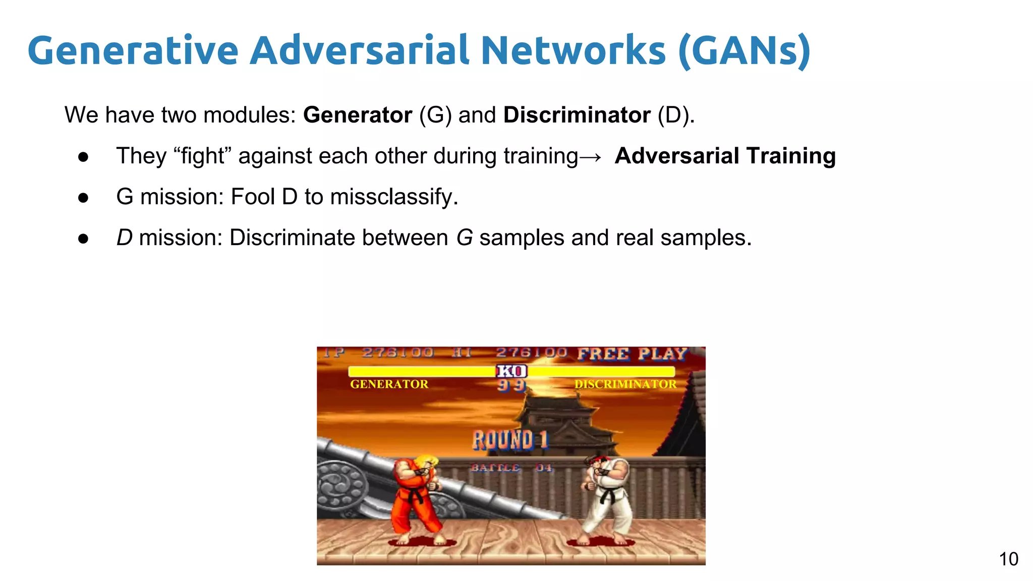
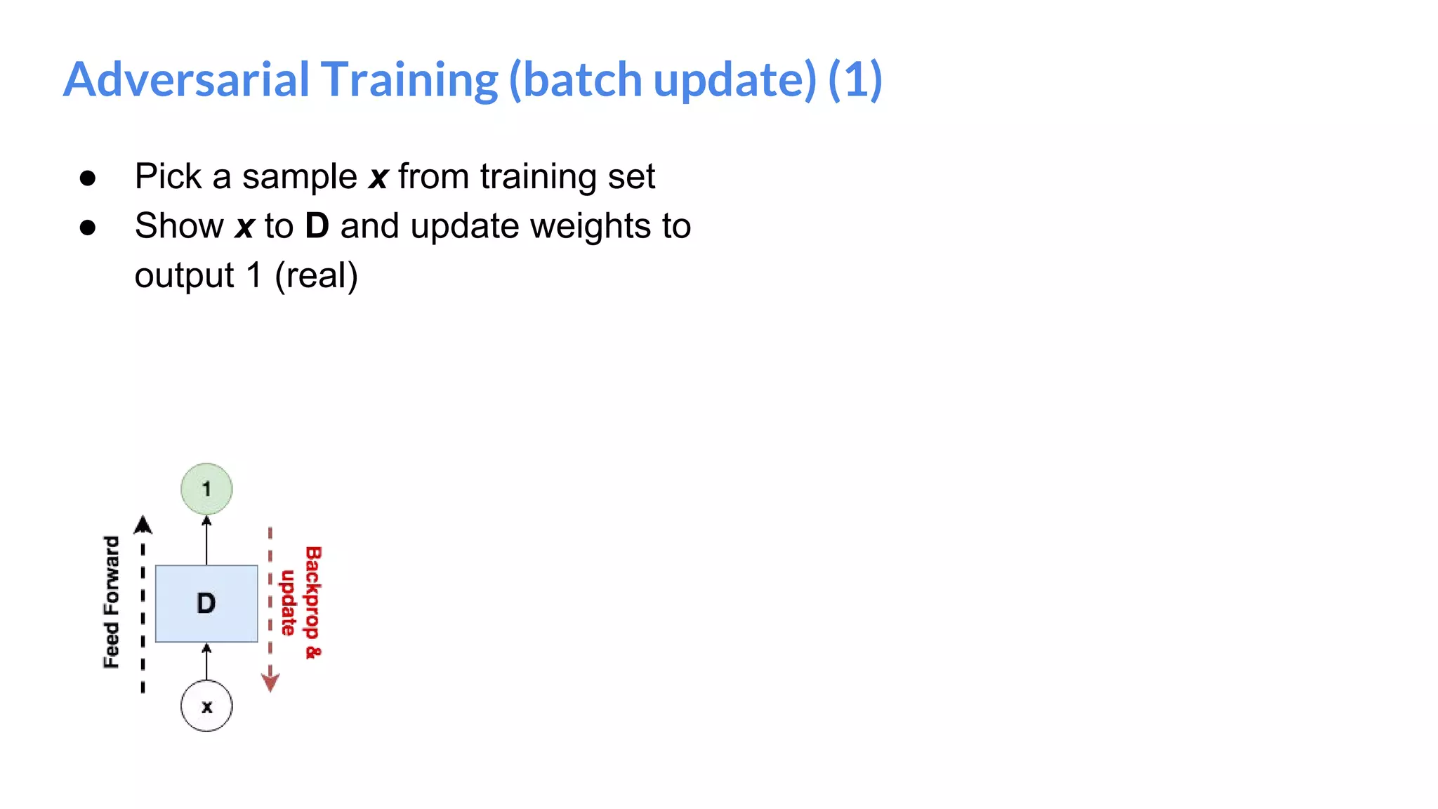
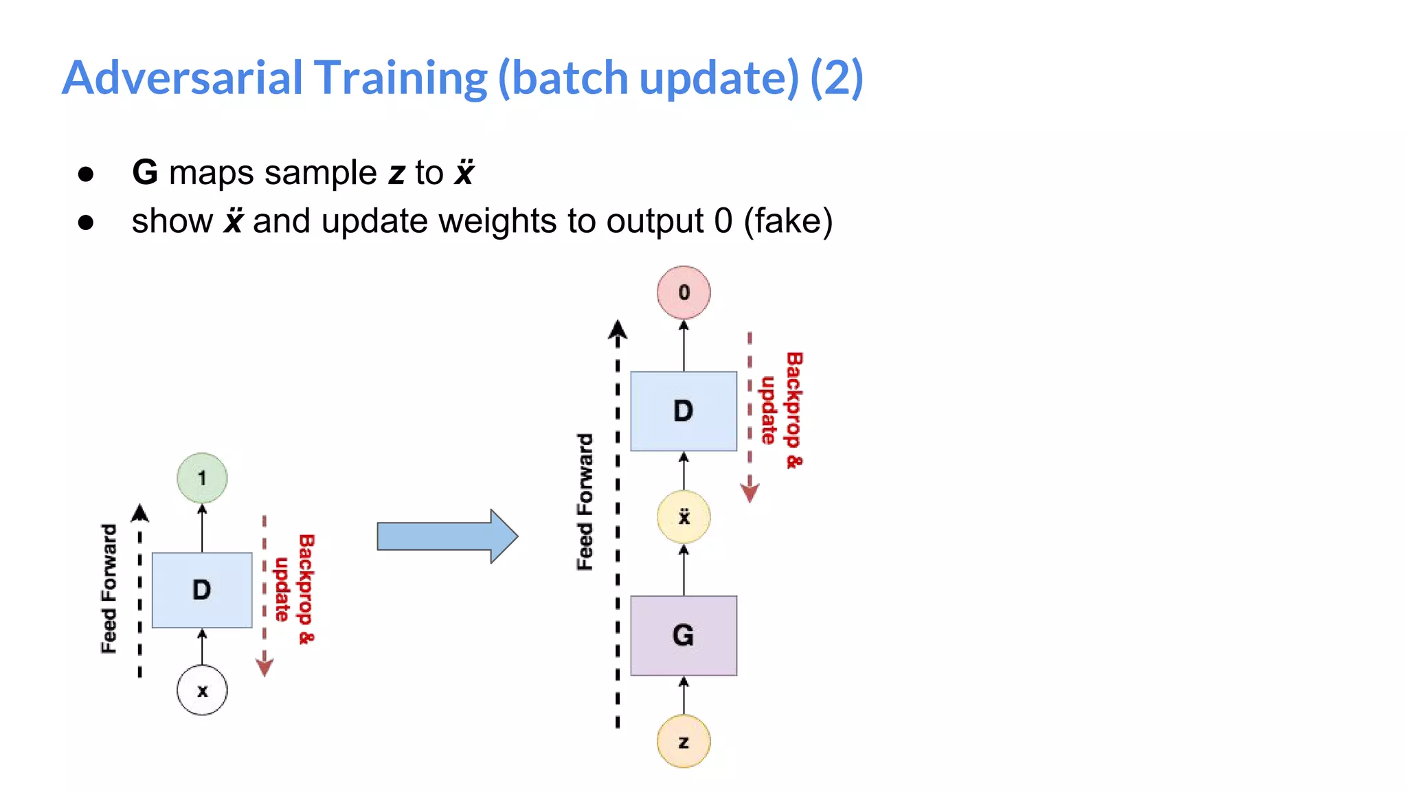
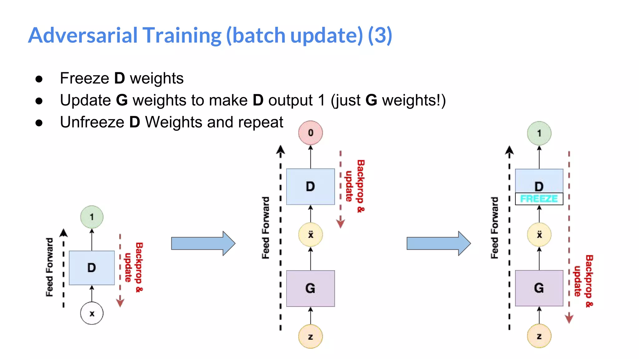
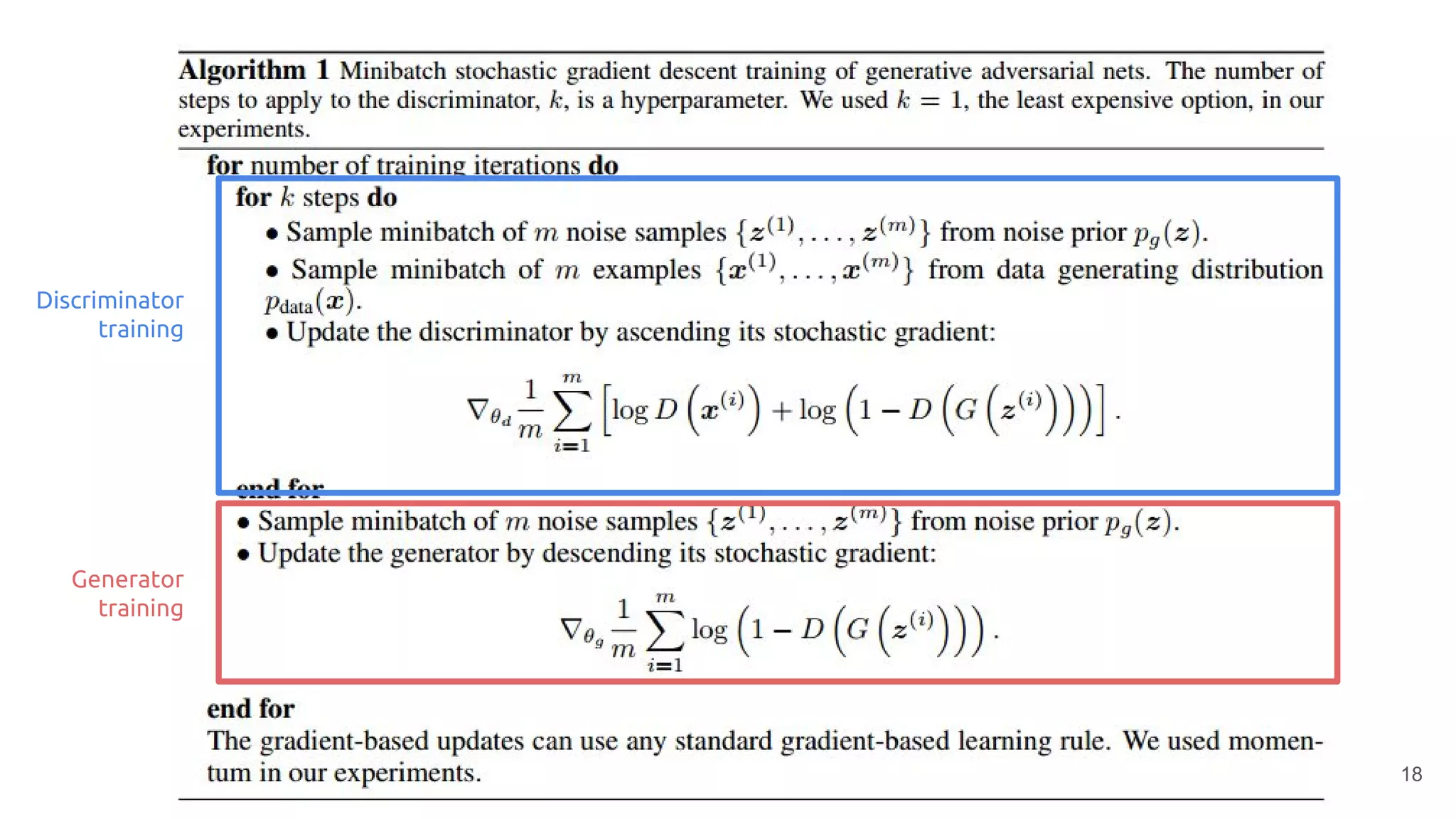
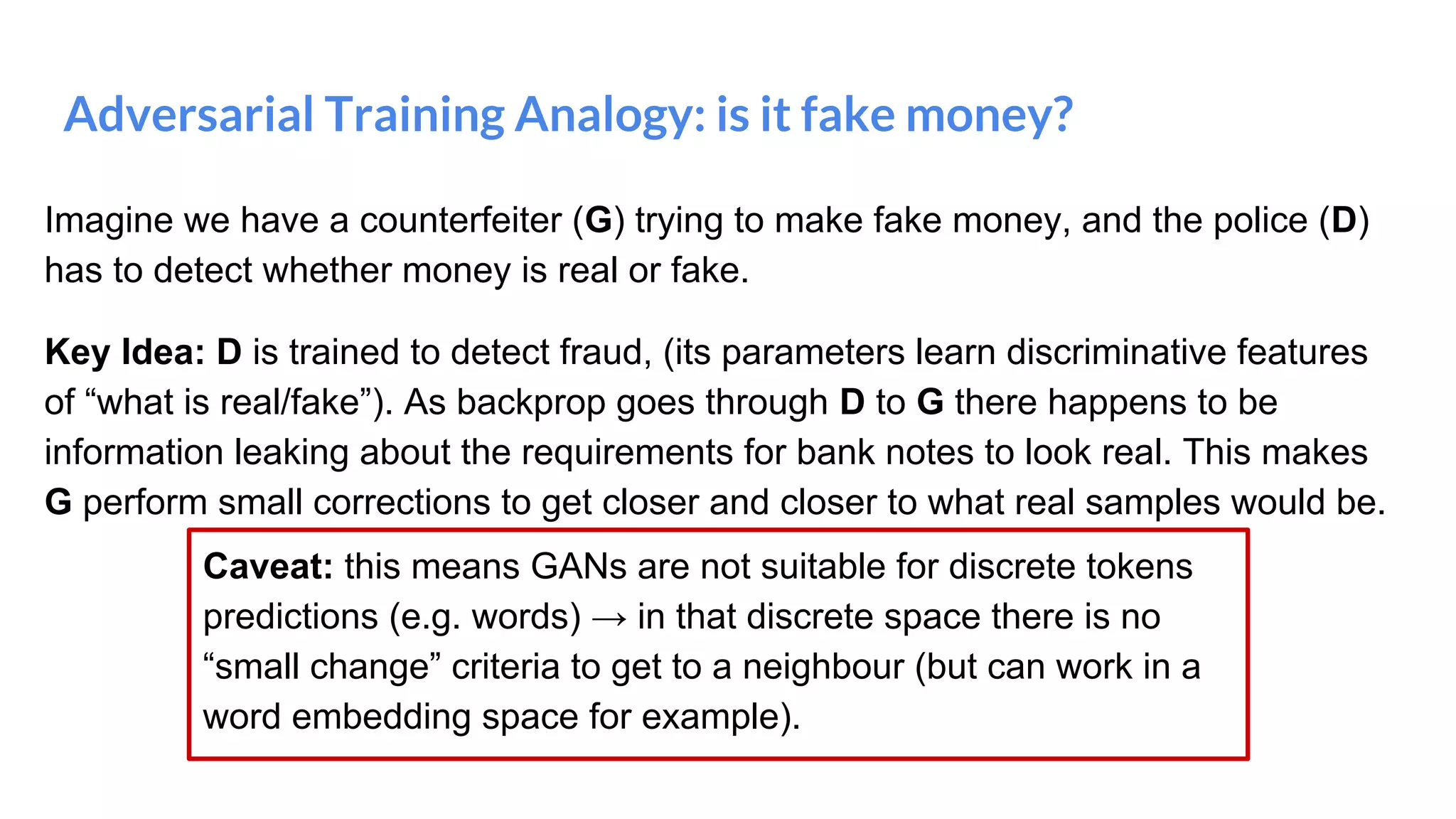
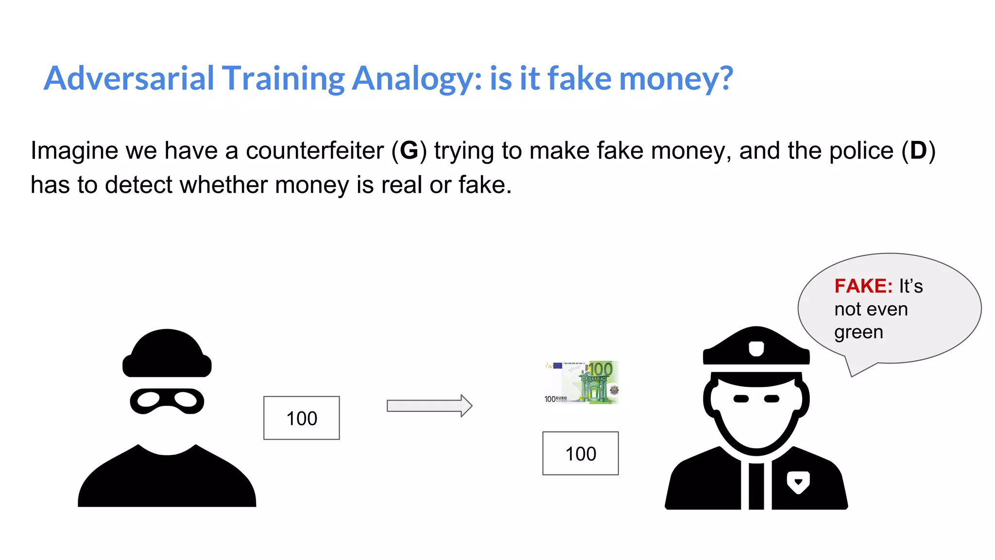
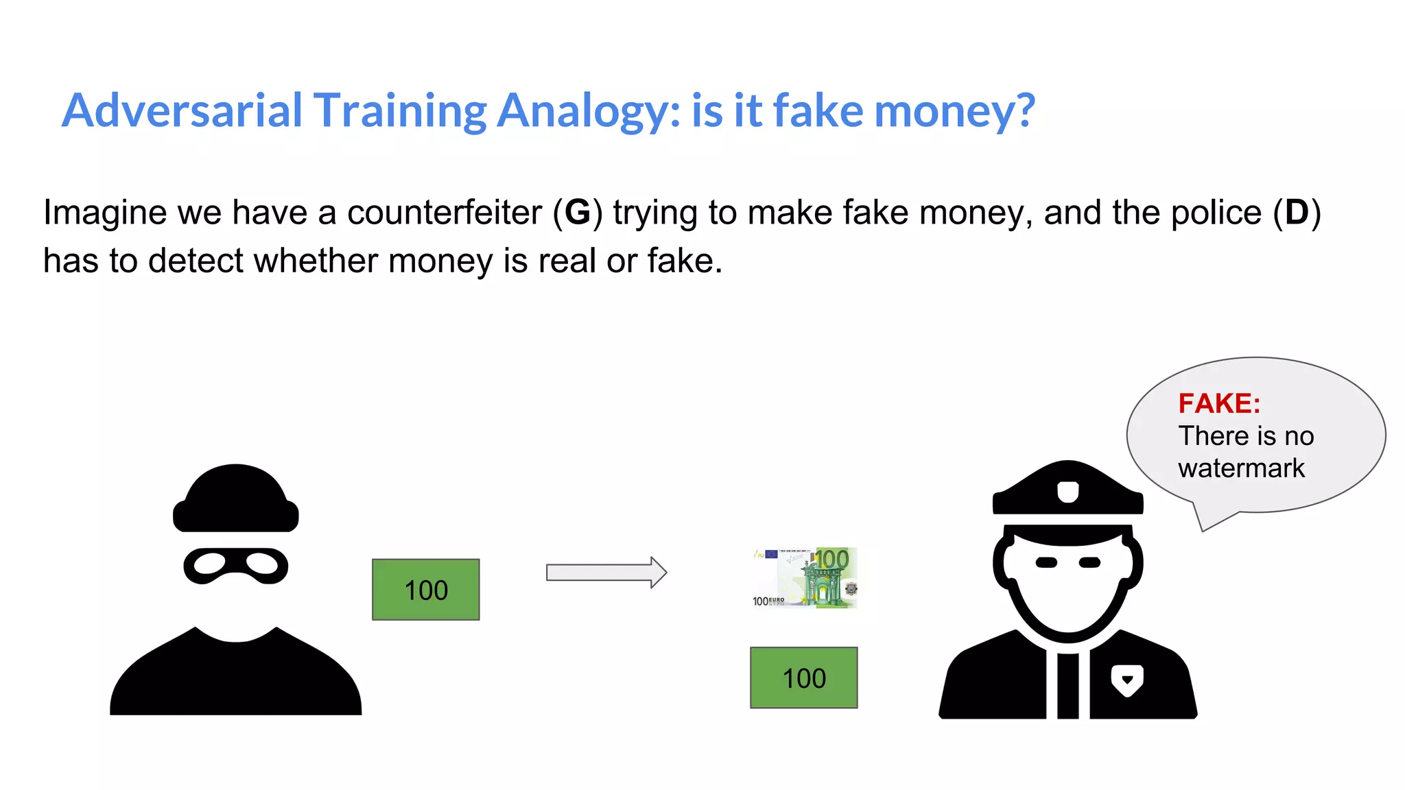
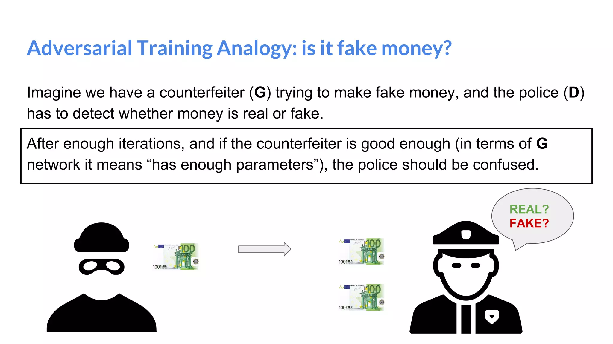
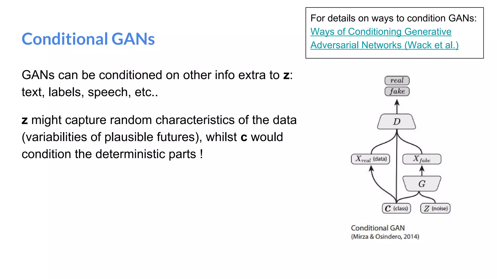
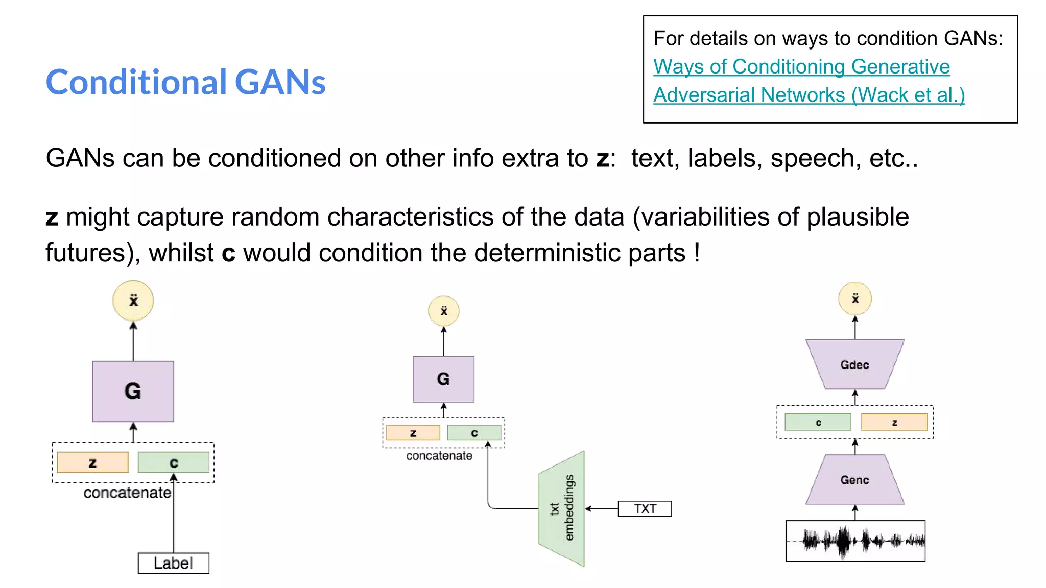
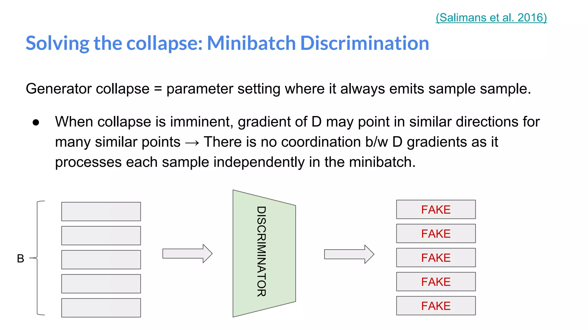
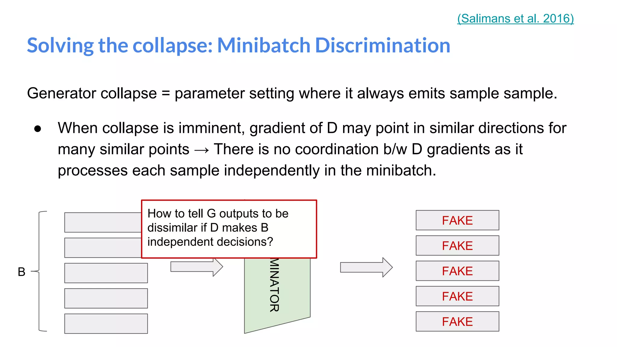
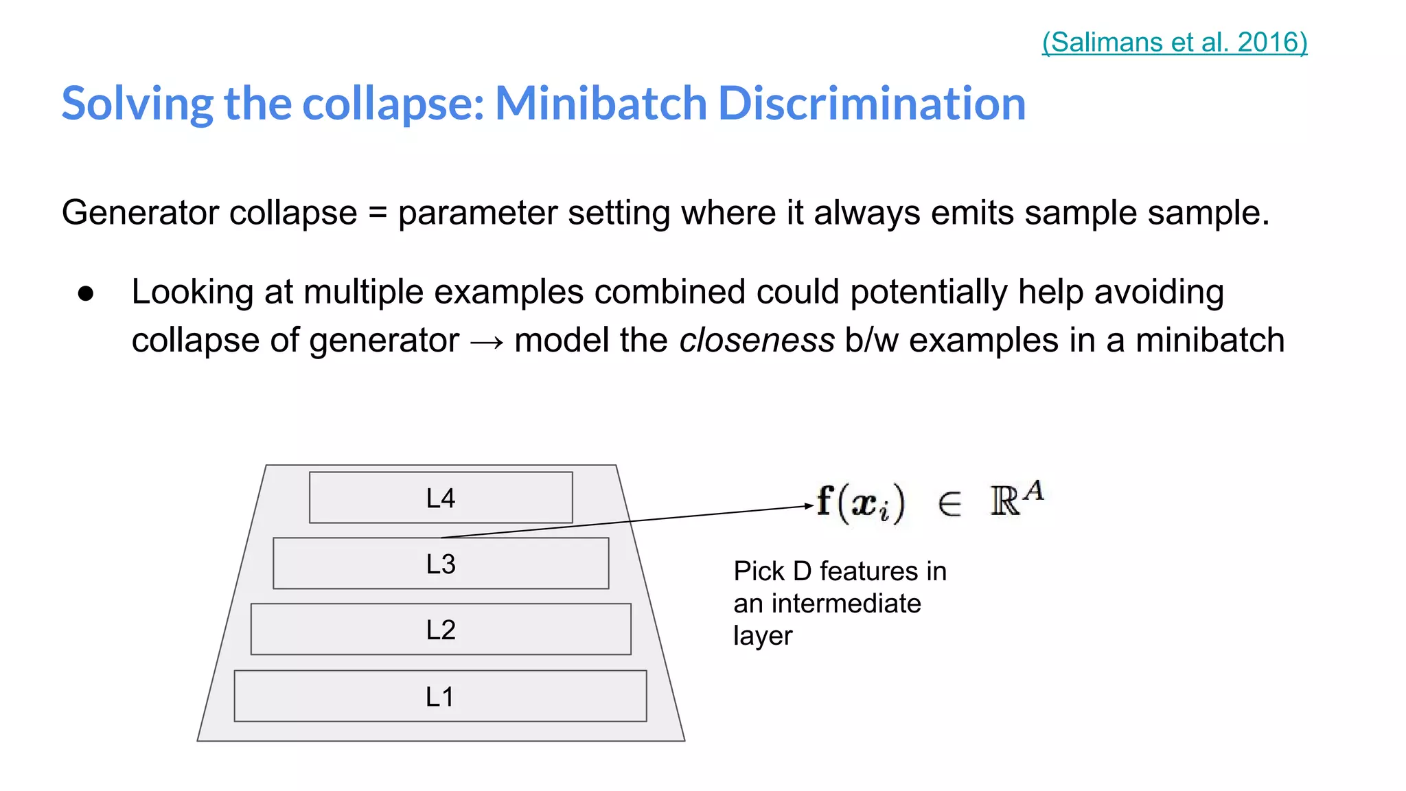
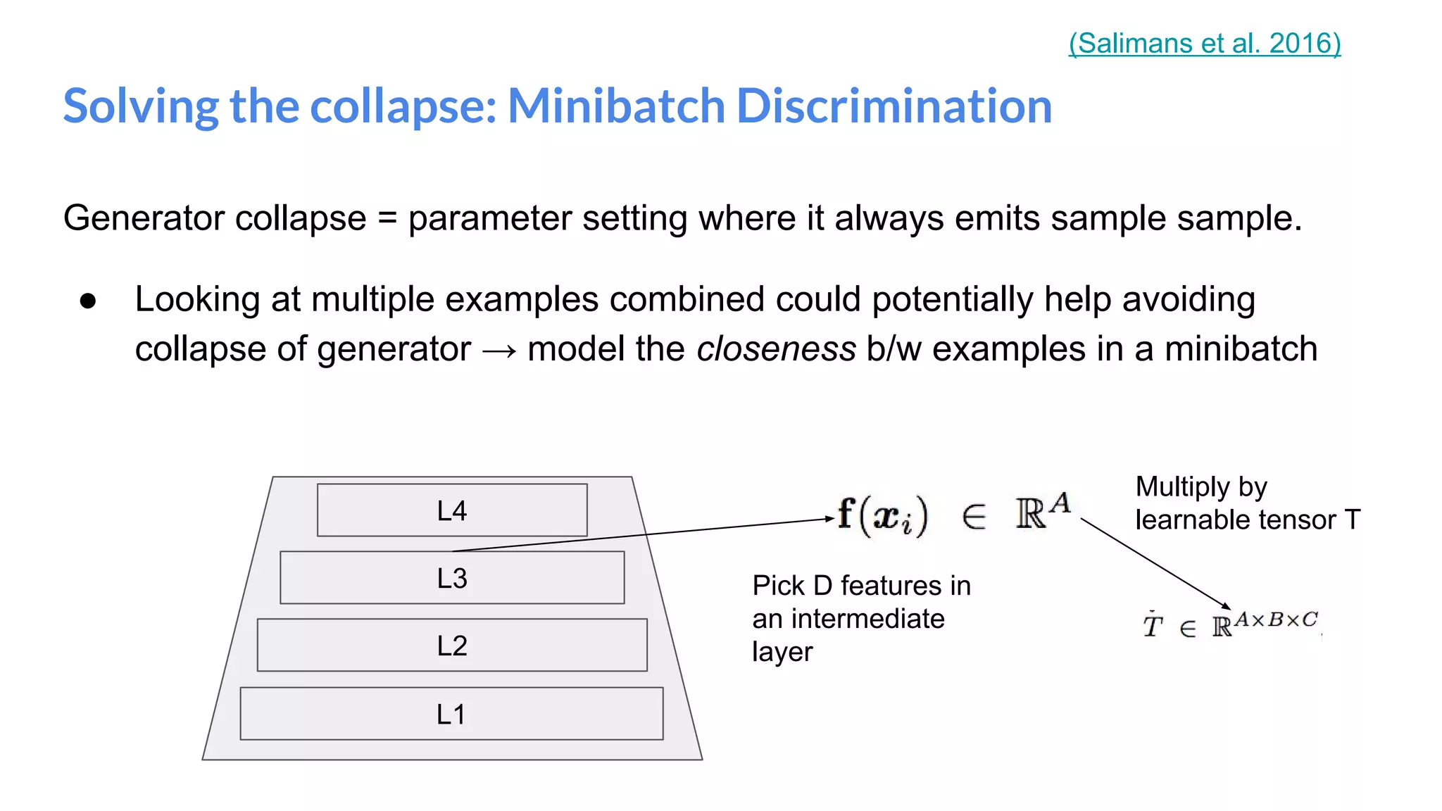
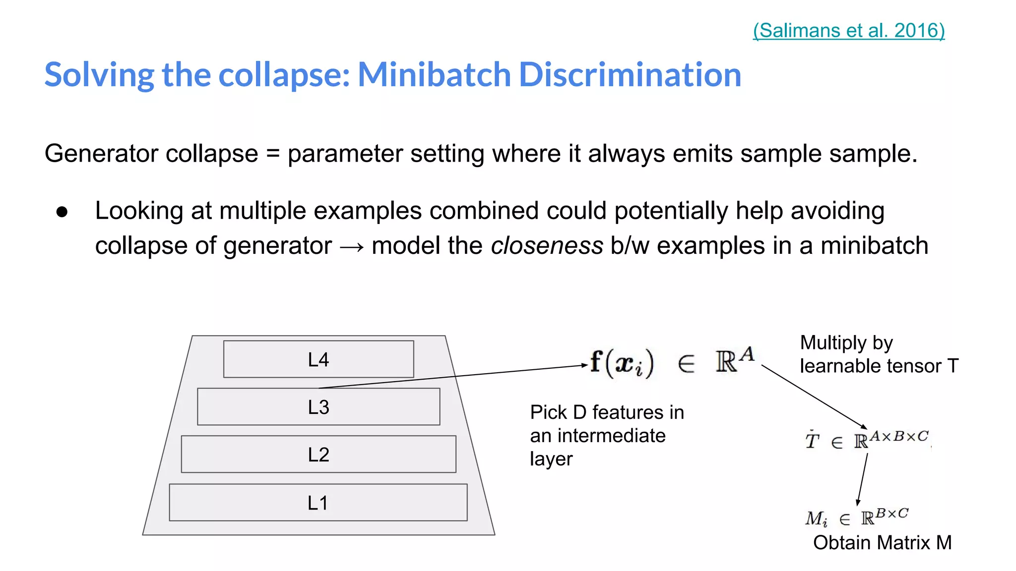
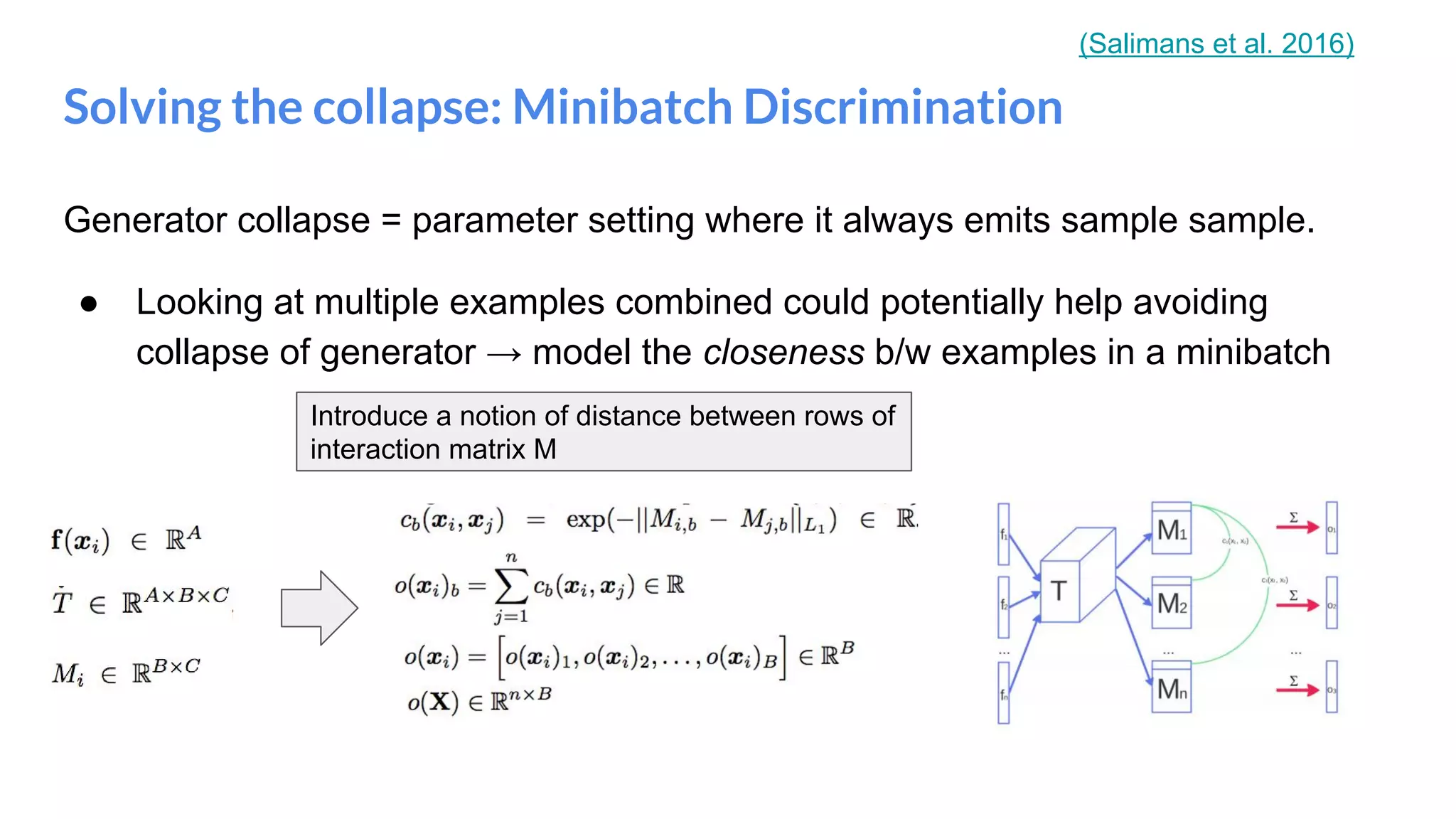
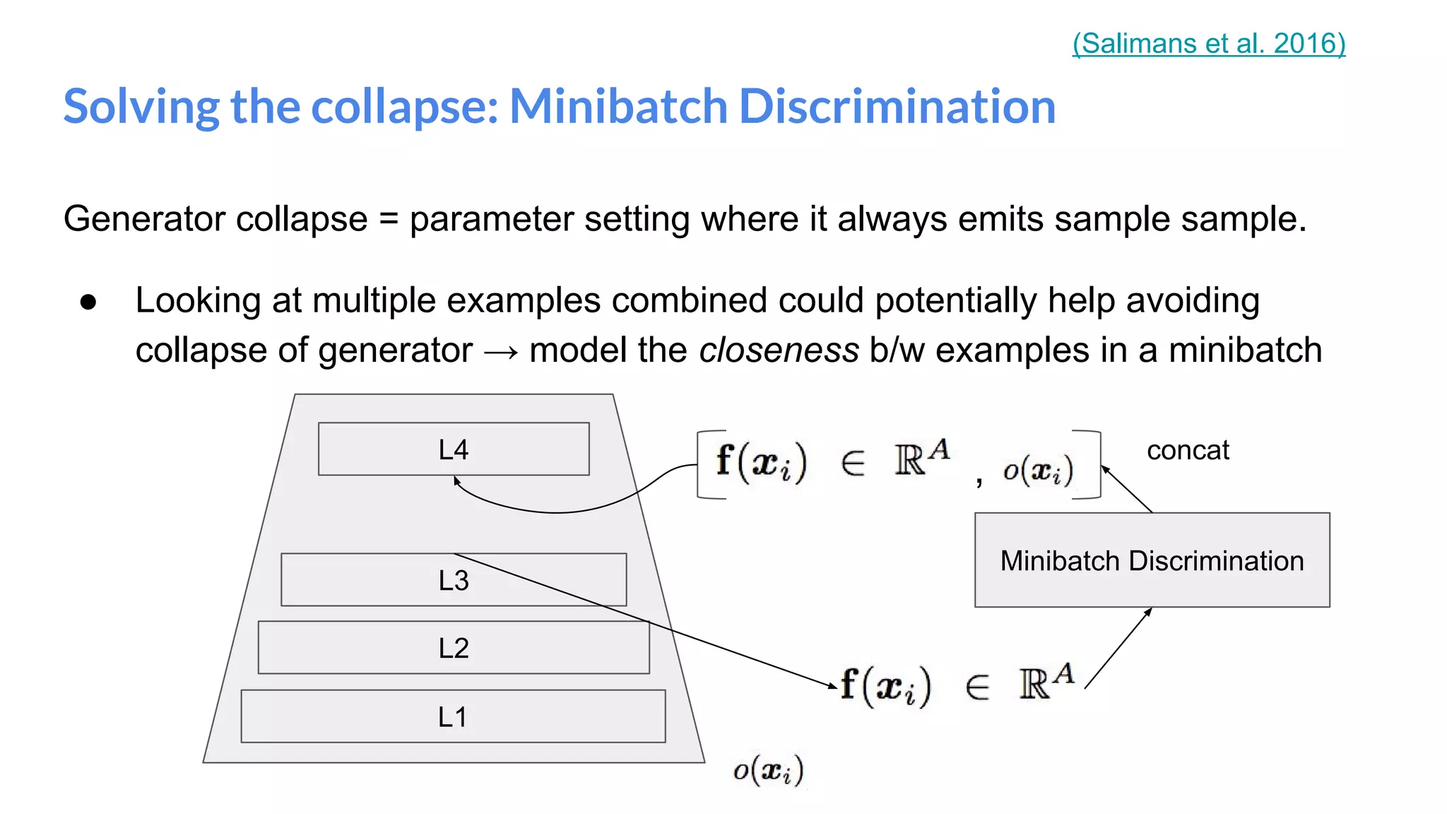
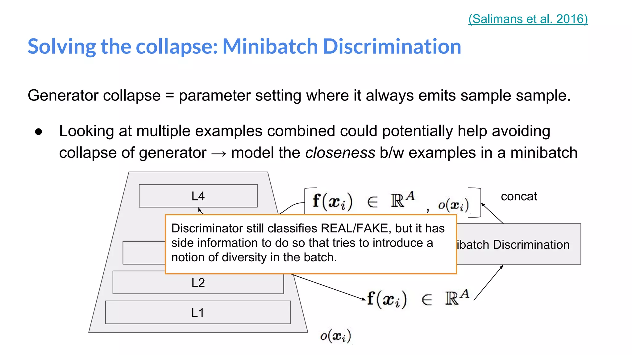
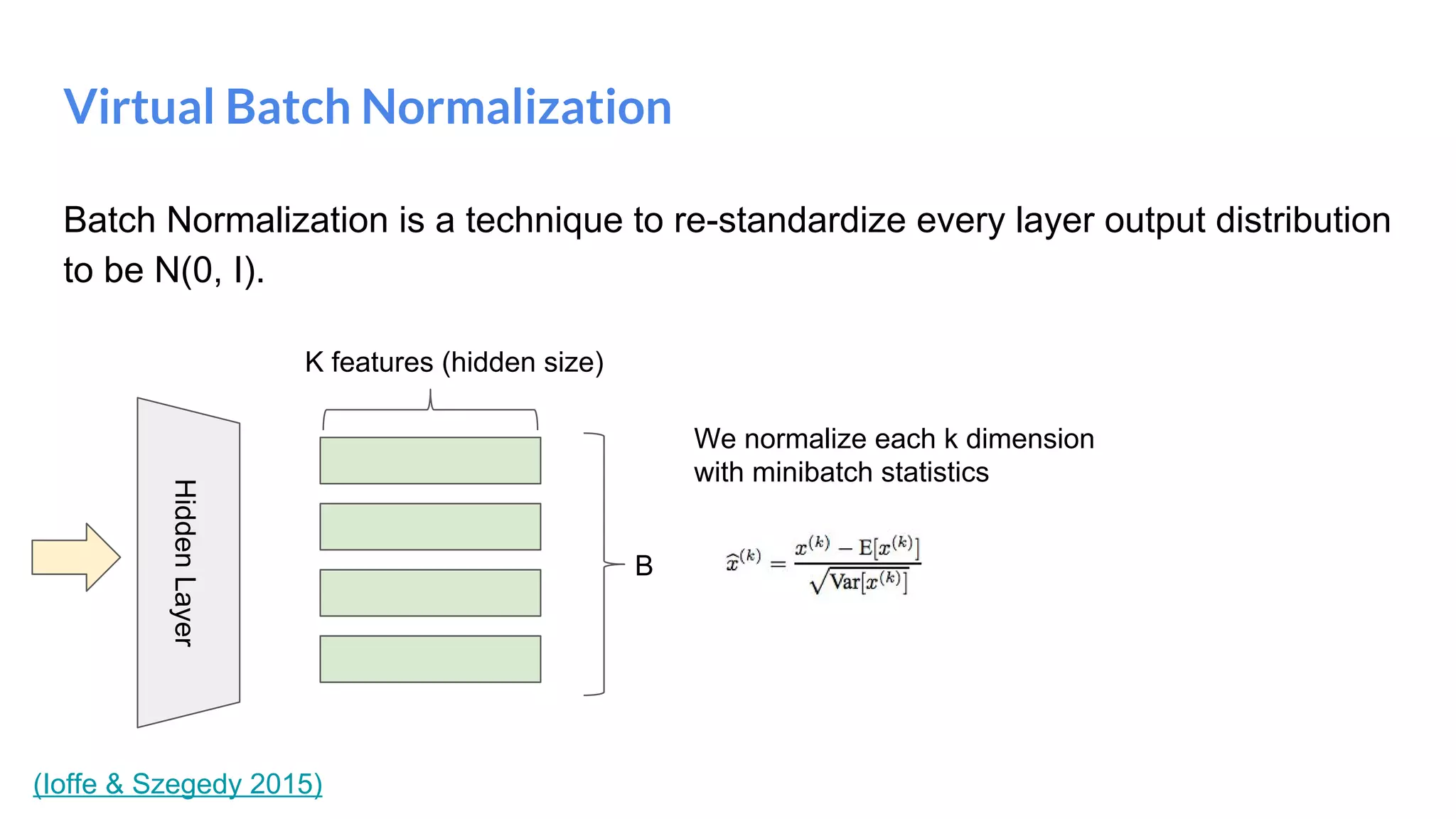
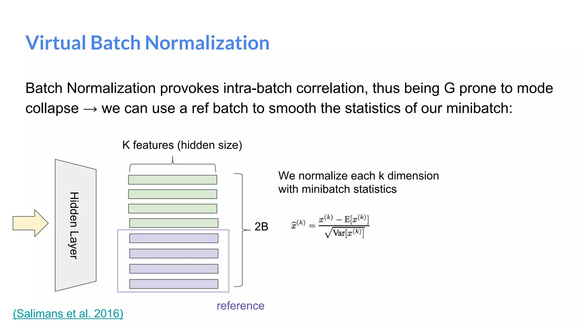
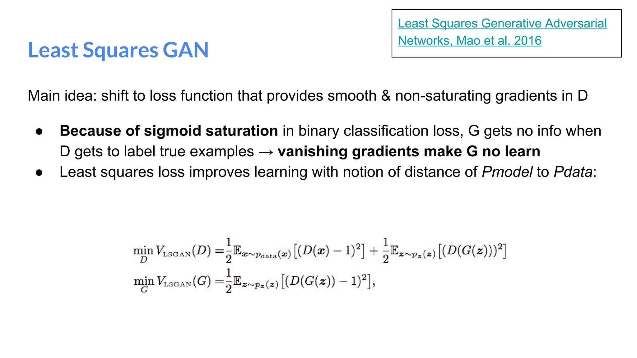
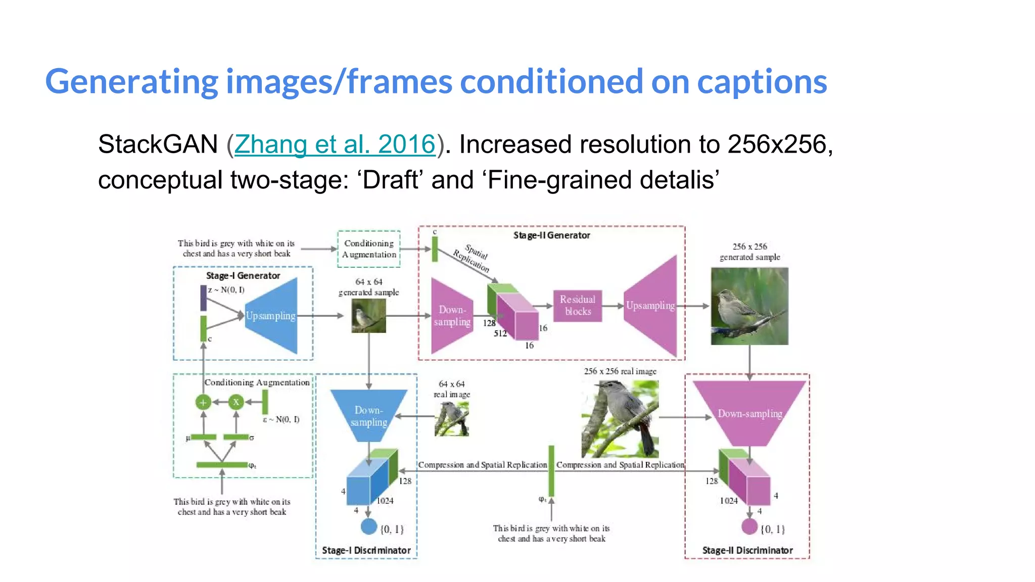
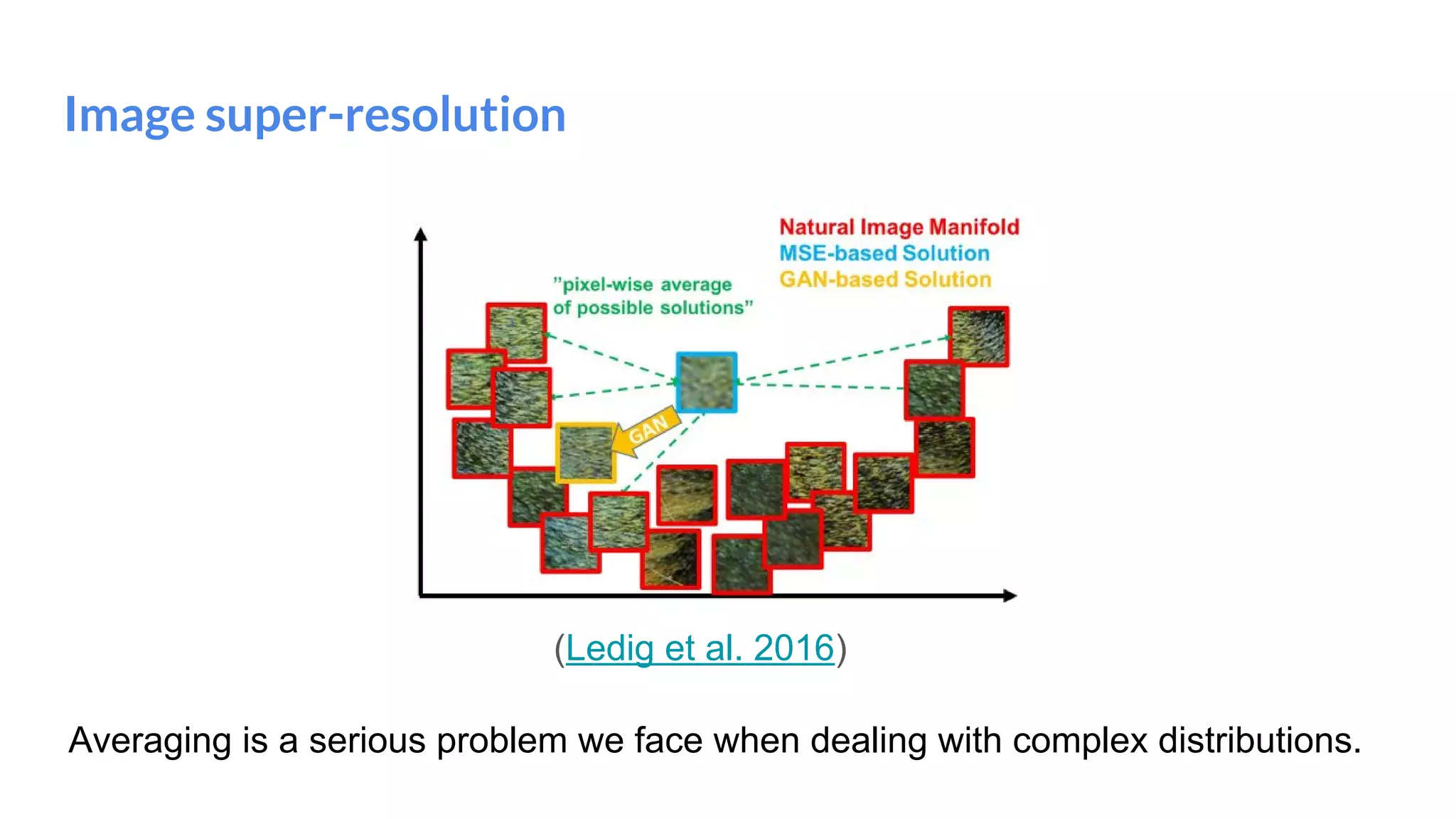
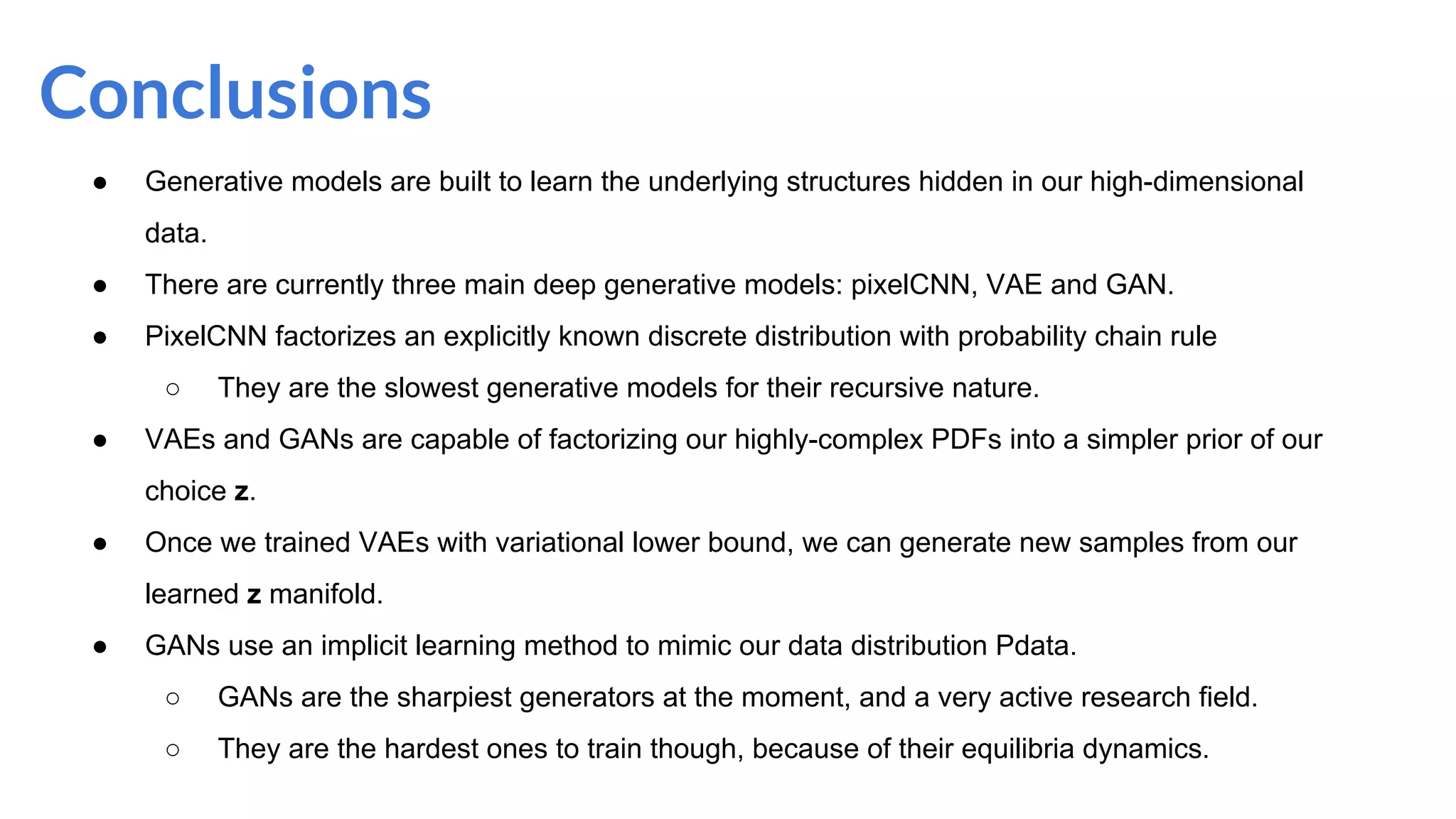
The document outlines a lecture on deep generative models, focusing on PixelCNN, Variational Autoencoders (VAEs), and Generative Adversarial Networks (GANs). It explains the mechanics of these models, including their training processes, advantages, and challenges, particularly the intricate dynamics of GAN training. The conclusion emphasizes the significance of generative models in learning complex data distributions and highlights GANs as leading generators despite their training difficulties.