Download to read offline
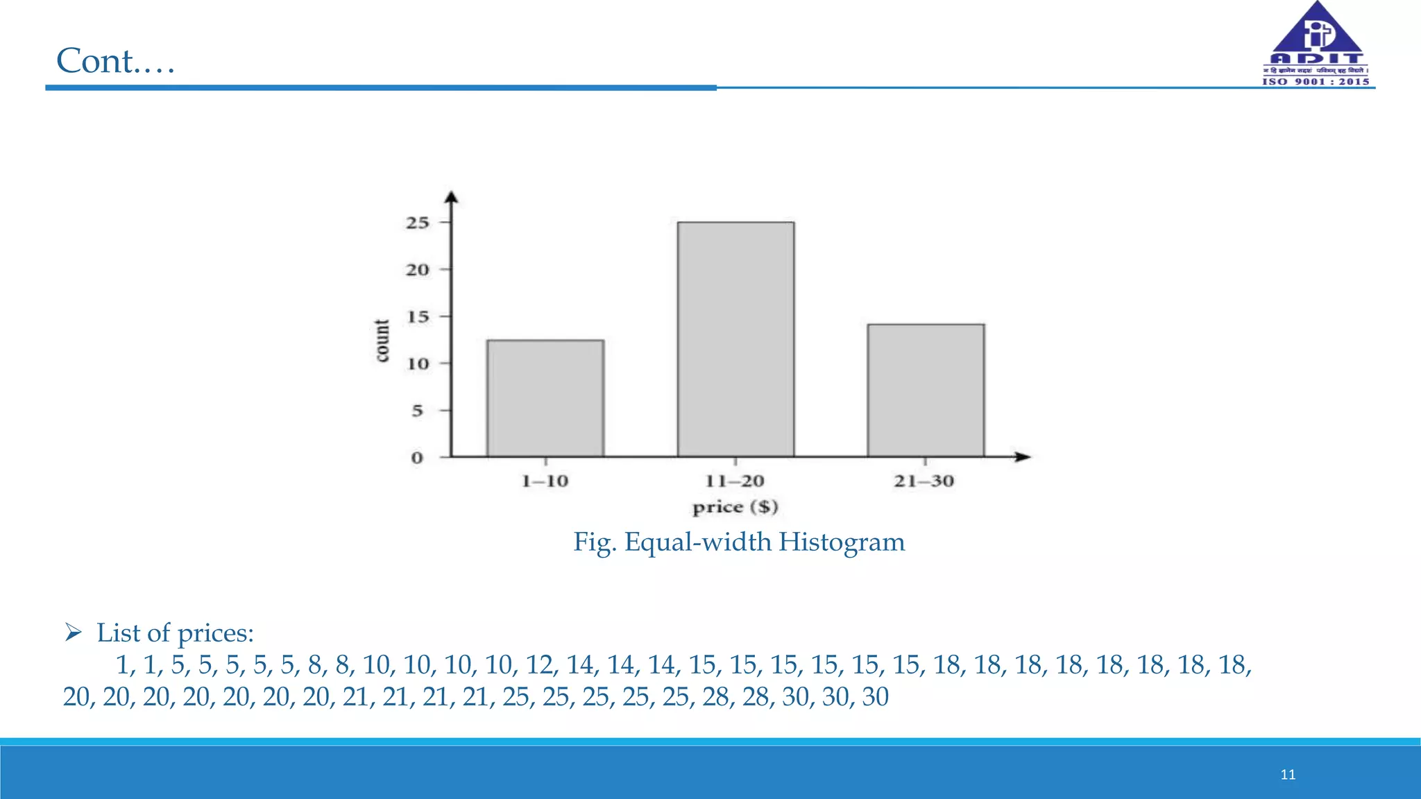
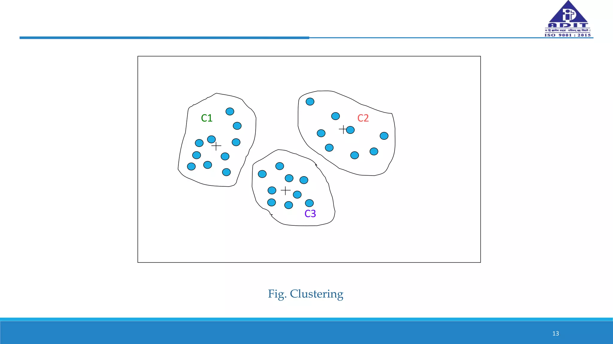
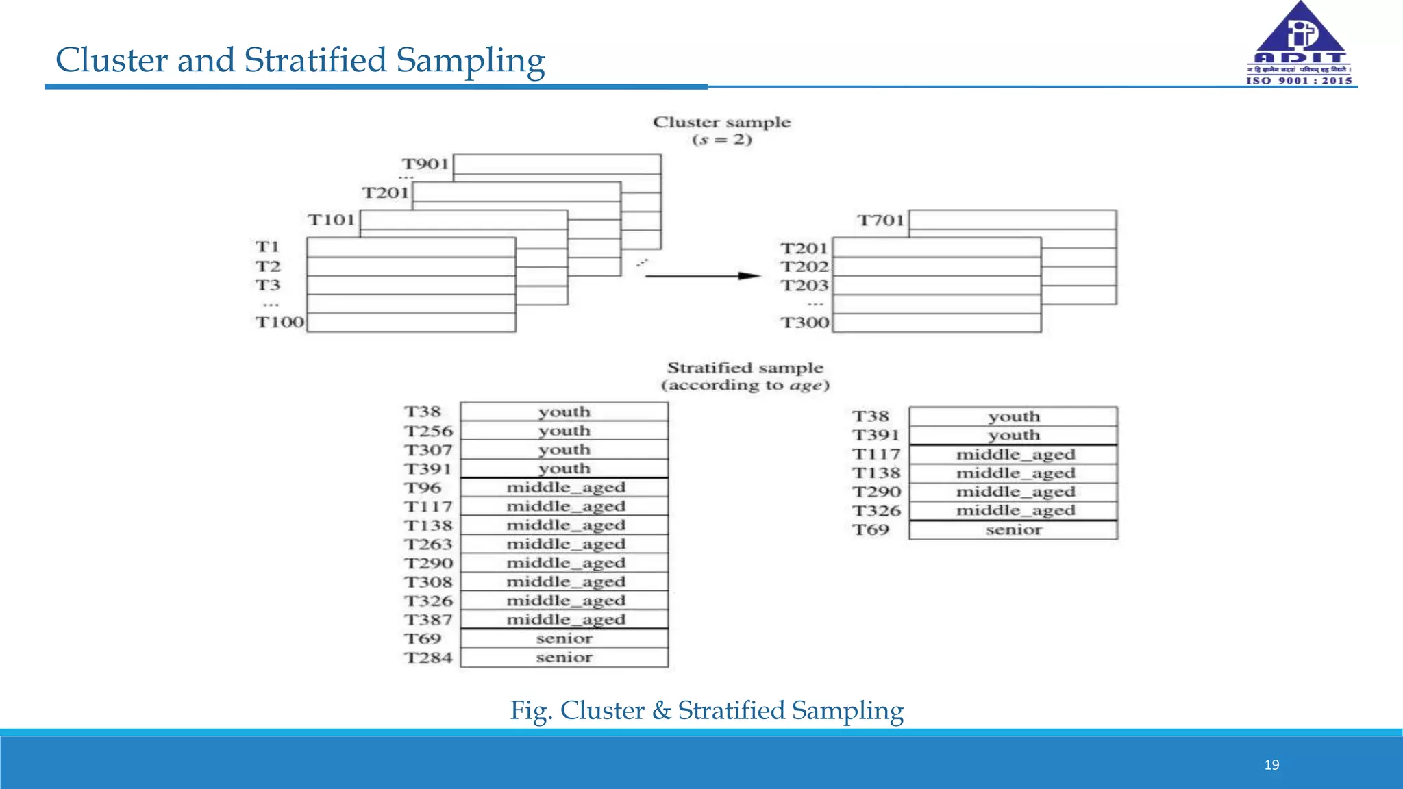
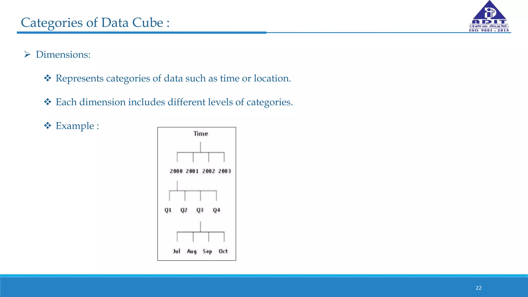
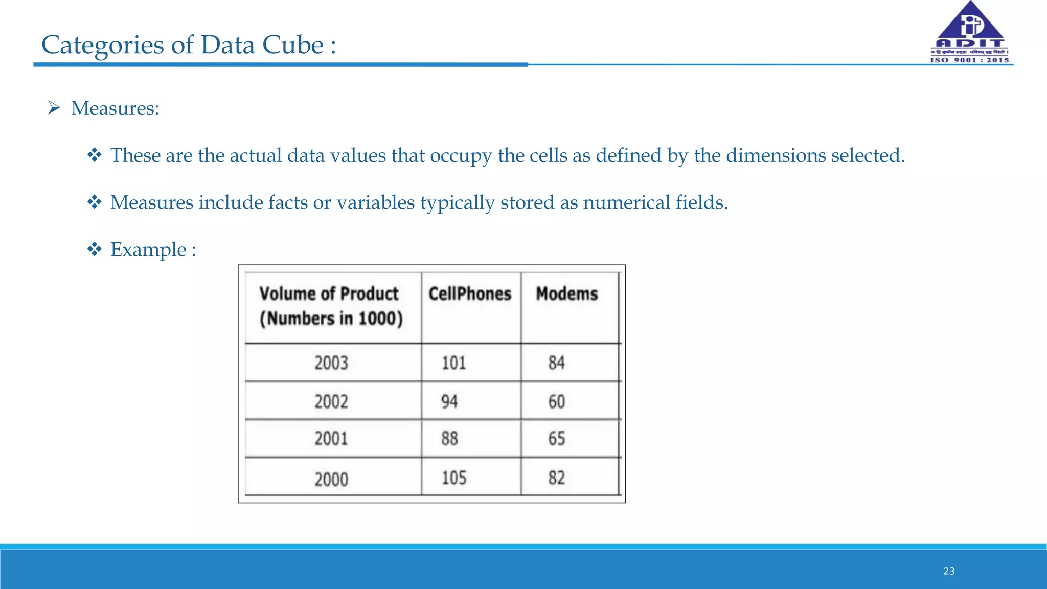


This document discusses various techniques for numerosity reduction in data mining. Numerosity reduction aims to reduce the volume of data while maintaining integrity. Methods include parametric approaches like regression and log-linear models, and non-parametric methods such as histograms, clustering, sampling, and data cube aggregation. Histograms bin data into buckets to store average values, while clustering partitions data into groups. Sampling obtains a representative subset of data. Data cube aggregation precomputes and stores multidimensional summarized data. Together, these techniques provide more efficient analysis of large datasets.