Downloaded 449 times
![26
of
39
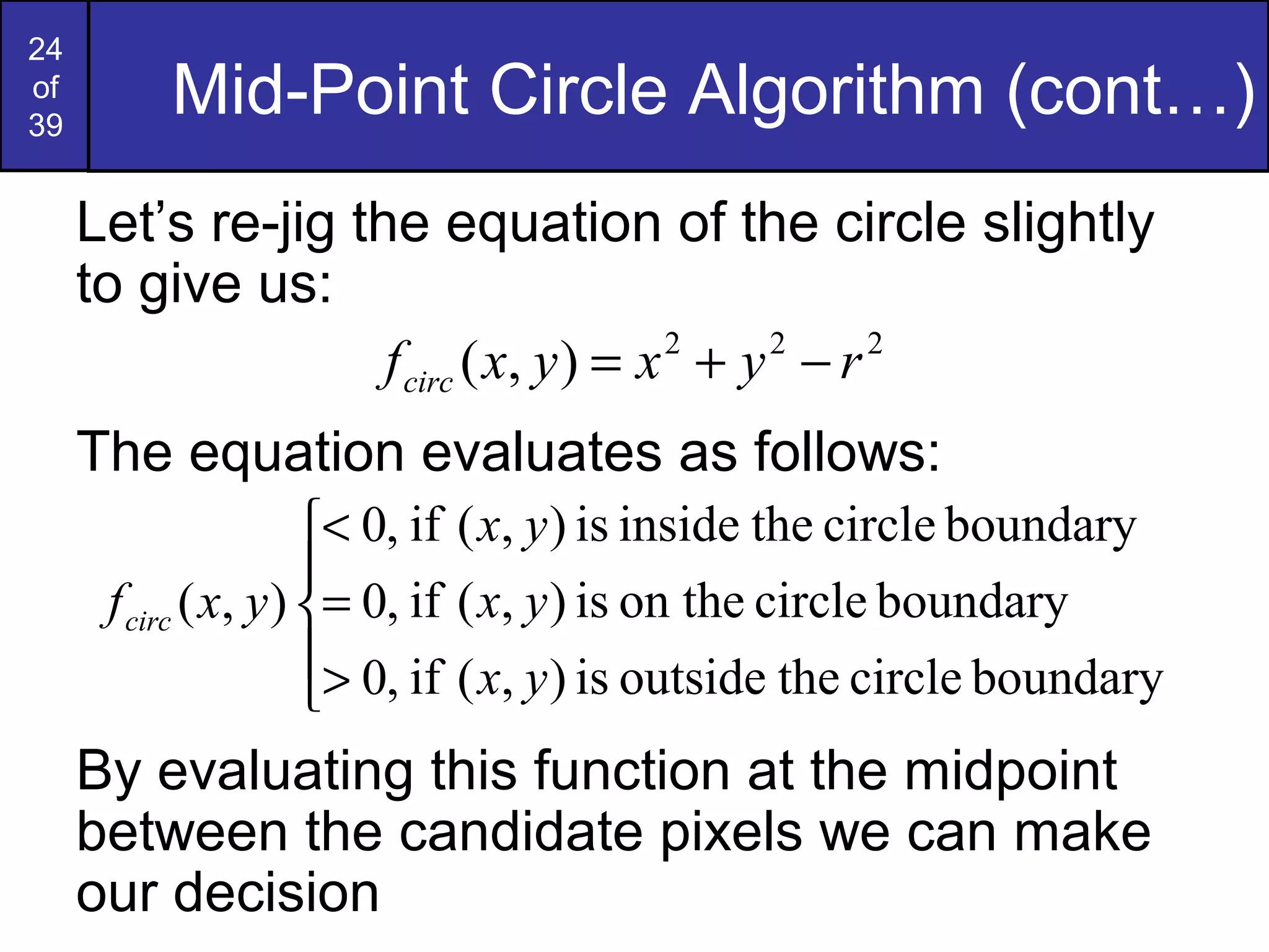
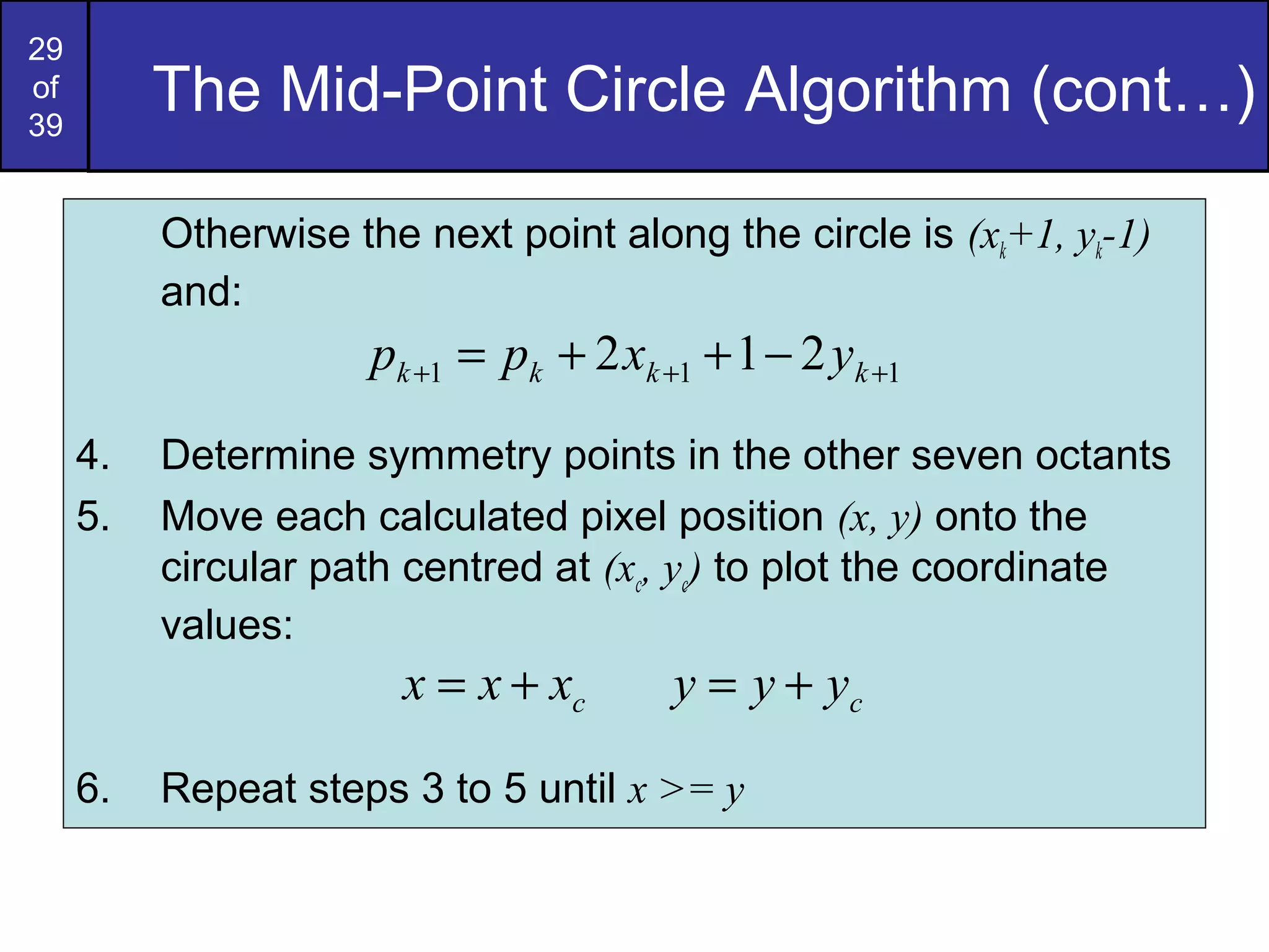
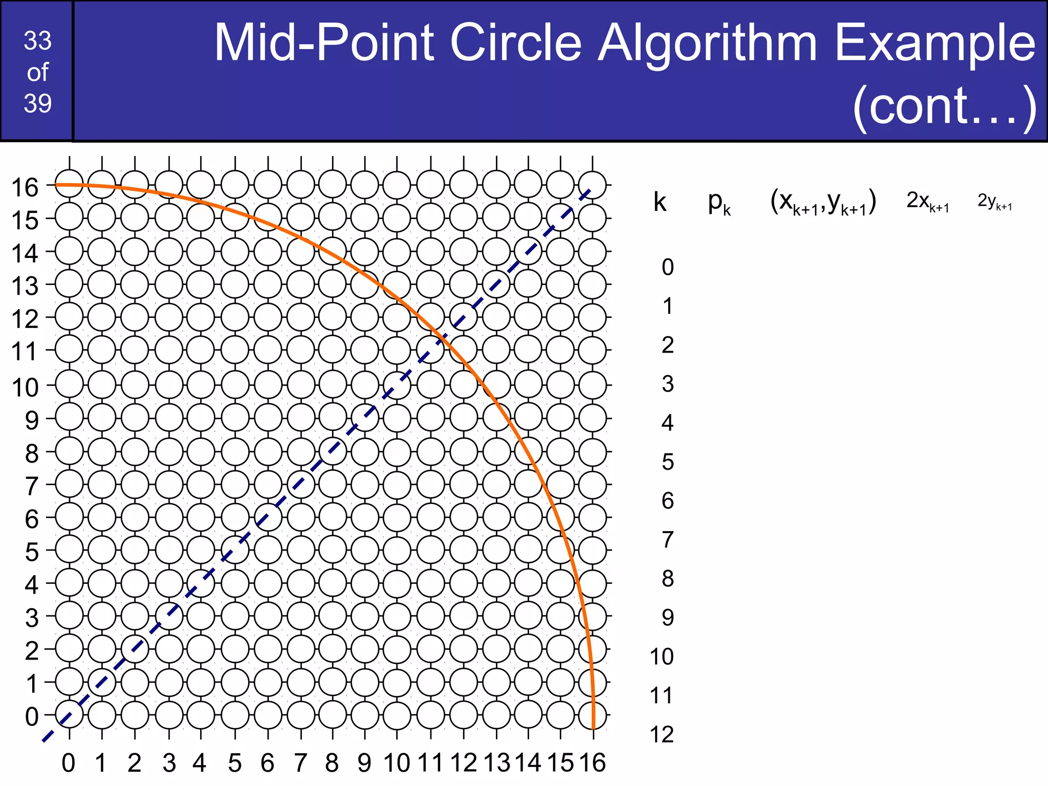
Mid-Point Circle Algorithm (cont…)
To ensure things are as efficient as possible
we can do all of our calculations
incrementally
First consider:
or:
where yk+1 is either yk or yk-1 depending on
the sign of p
( )
( ) 2
2
1
2
111
2
1]1)1[(
2
1,1
ryx
yxfp
kk
kkcirck
−−+++=
−+=
+
+++
1)()()1(2 1
22
11 +−−−+++= +++ kkkkkkk yyyyxpp](https://image.slidesharecdn.com/graphics6-bresenhamcirclesandpolygons-140727131614-phpapp01/75/bresenham-circles-and-polygons-in-computer-graphics-Computer-graphics-tutorials-26-2048.jpg)


![26
of
39
Mid-Point Circle Algorithm (cont…)
To ensure things are as efficient as possible
we can do all of our calculations
incrementally
First consider:
or:
where yk+1 is either yk or yk-1 depending on
the sign of p
( )
( ) 2
2
1
2
111
2
1]1)1[(
2
1,1
ryx
yxfp
kk
kkcirck
−−+++=
−+=
+
+++
1)()()1(2 1
22
11 +−−−+++= +++ kkkkkkk yyyyxpp](https://crownmelresort.com/image.slidesharecdn.com/graphics6-bresenhamcirclesandpolygons-140727131614-phpapp01/75/bresenham-circles-and-polygons-in-computer-graphics-Computer-graphics-tutorials-26-2048.jpg)


The document discusses various computer graphics algorithms, focusing on Bresenham's line drawing algorithm, mid-point circle algorithm, and polygon filling techniques. It details the steps and advantages of these algorithms, highlighting how they optimize drawing using integer calculations and symmetry. Additionally, it compares them with other methods like the DDA algorithm to illustrate their efficiency.
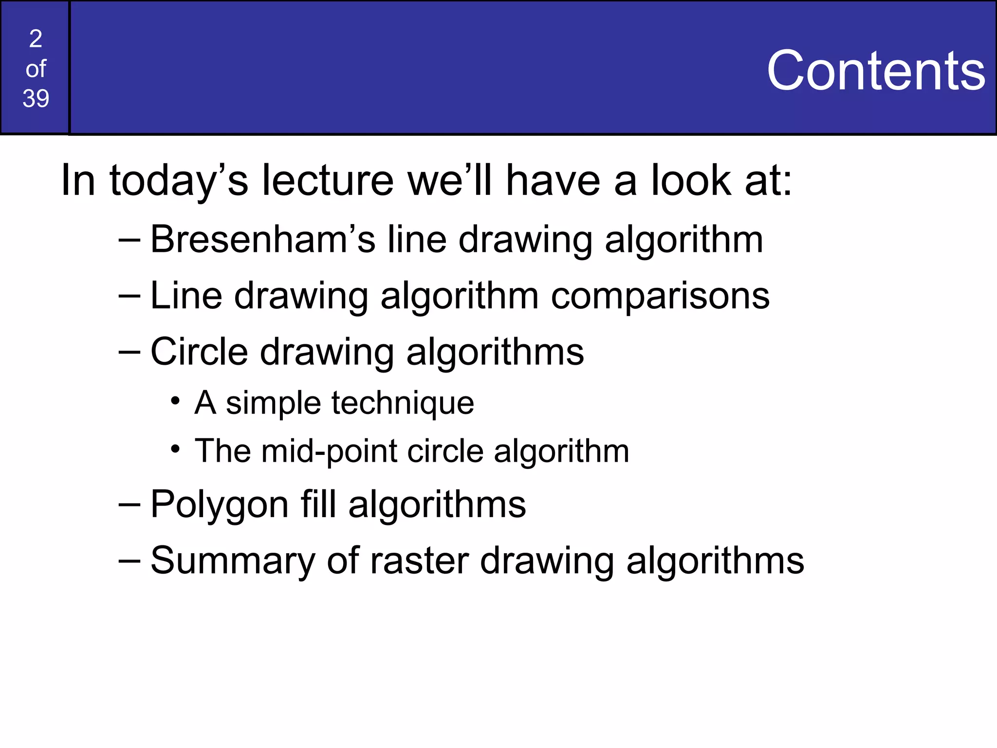
Overview of course topics, focusing on Bresenham's line algorithm, circle drawing, and polygon filling.
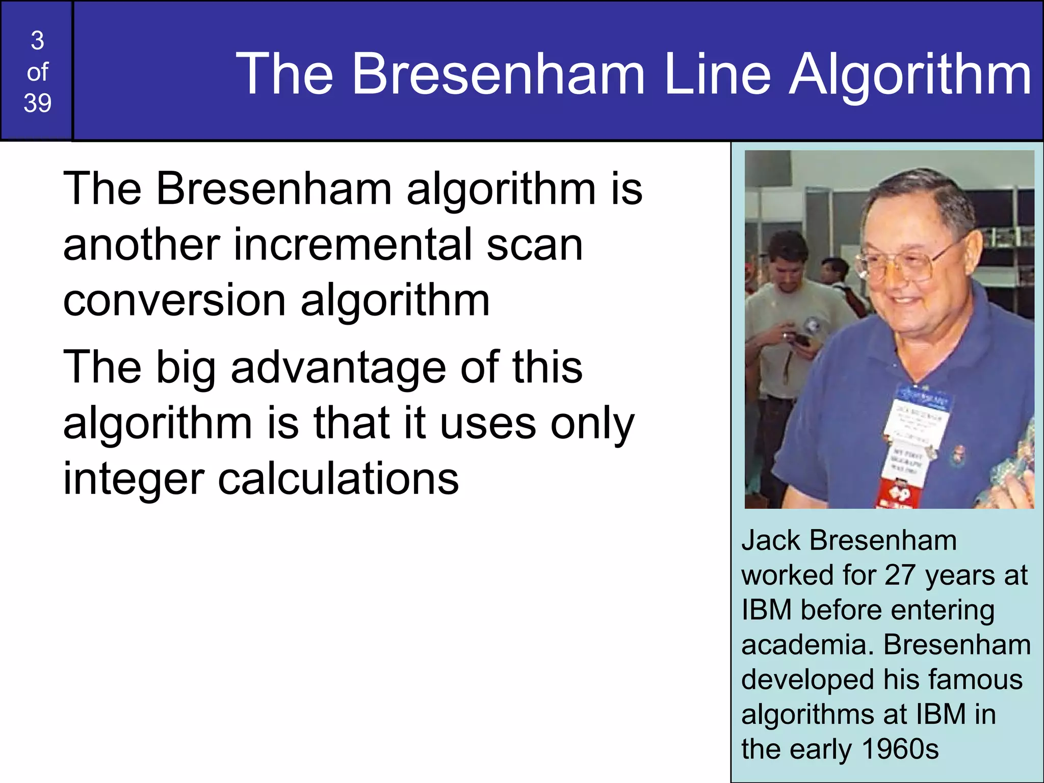
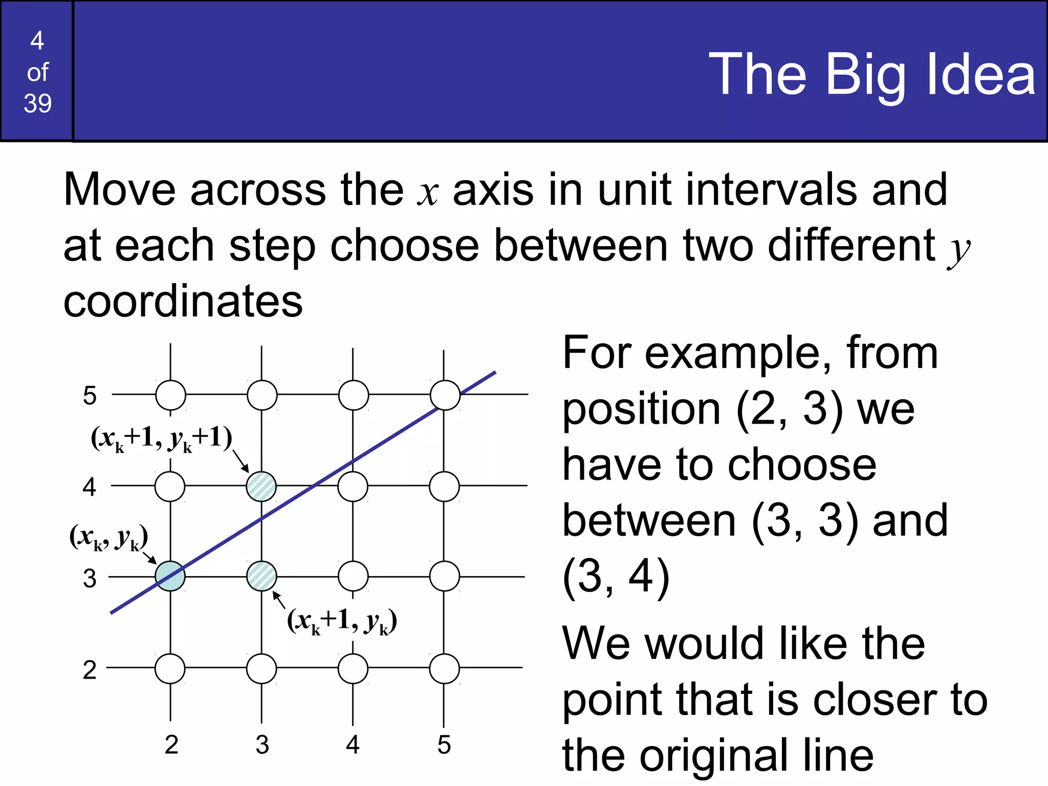
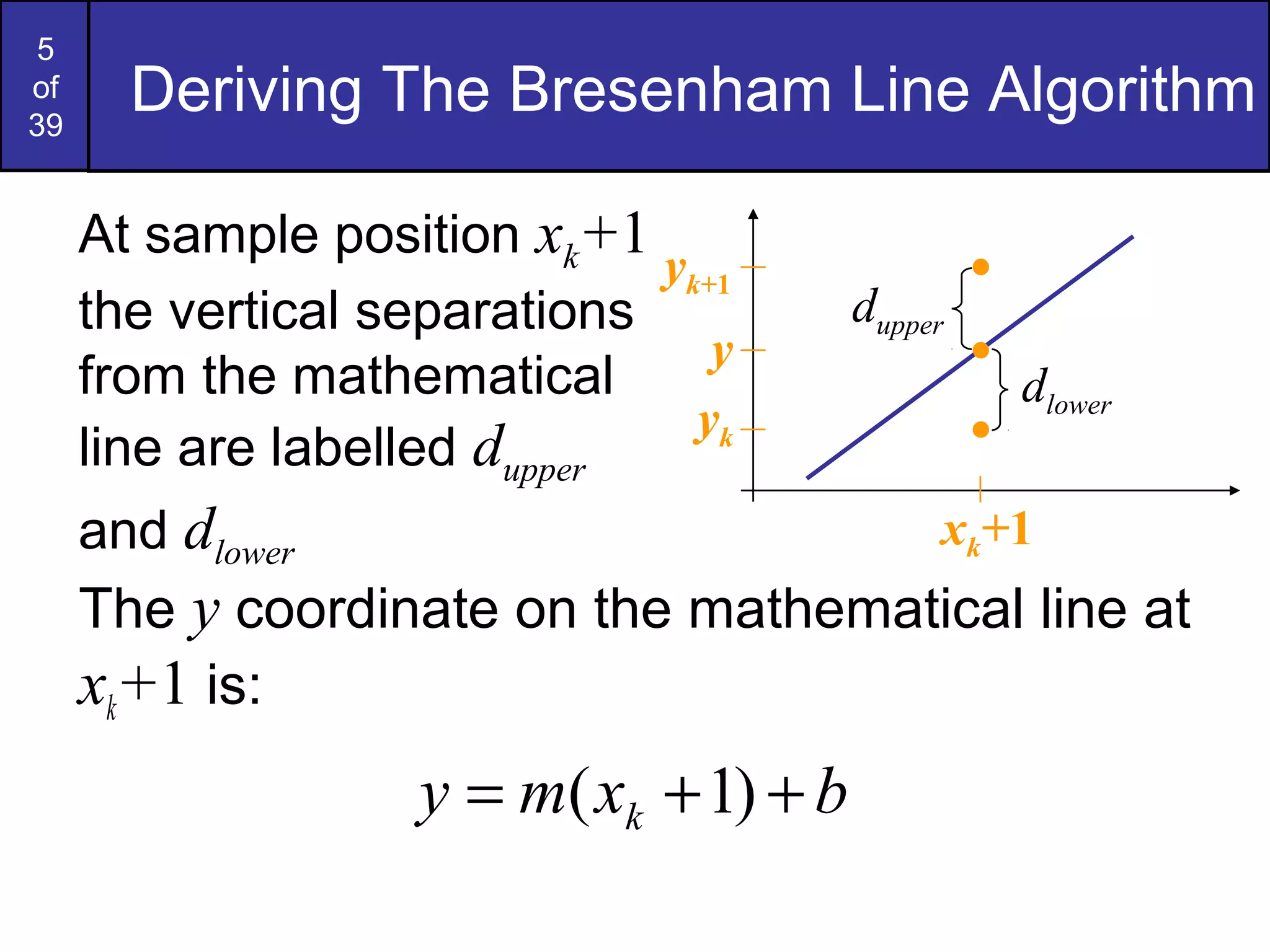
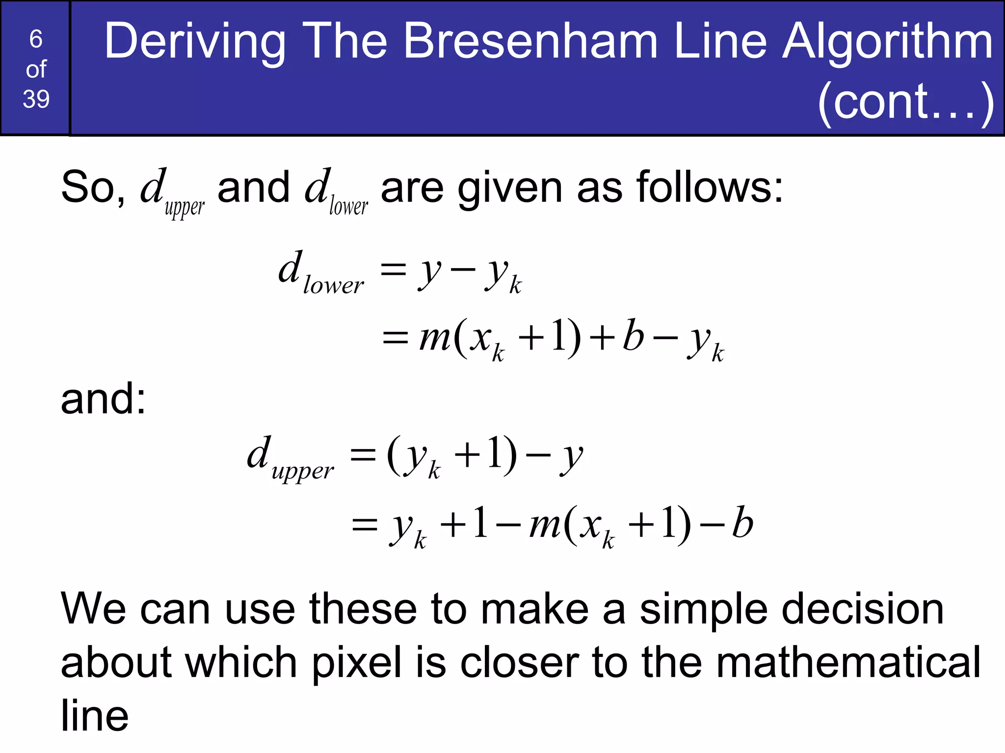
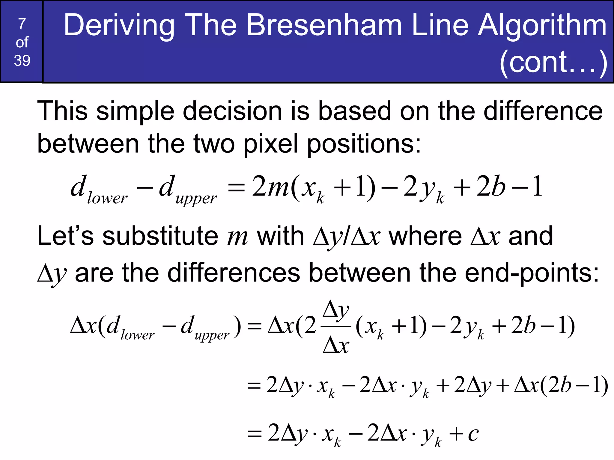
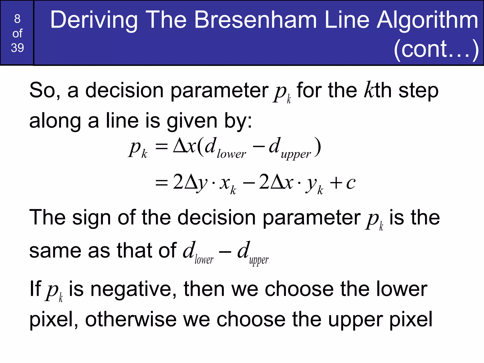
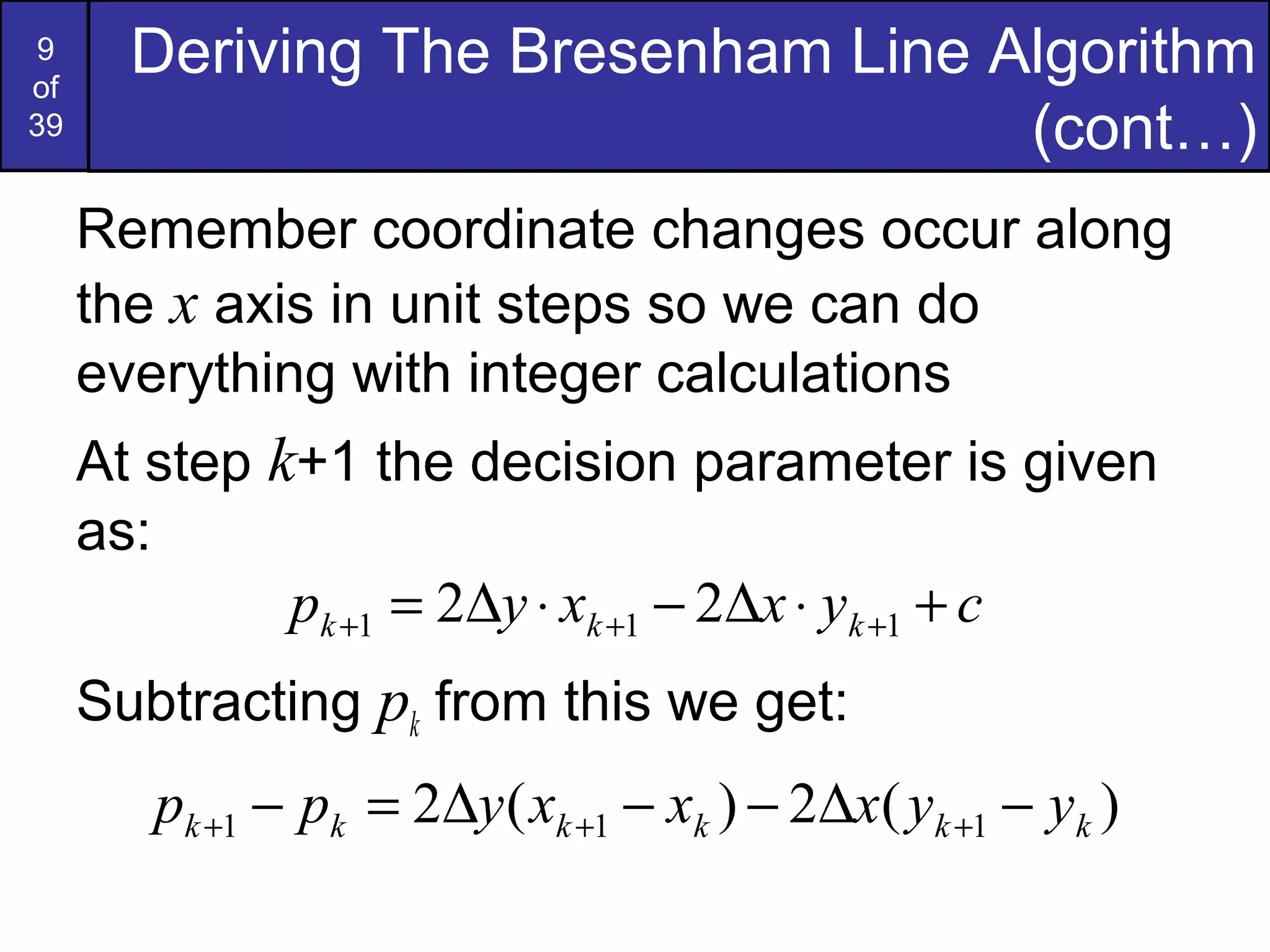
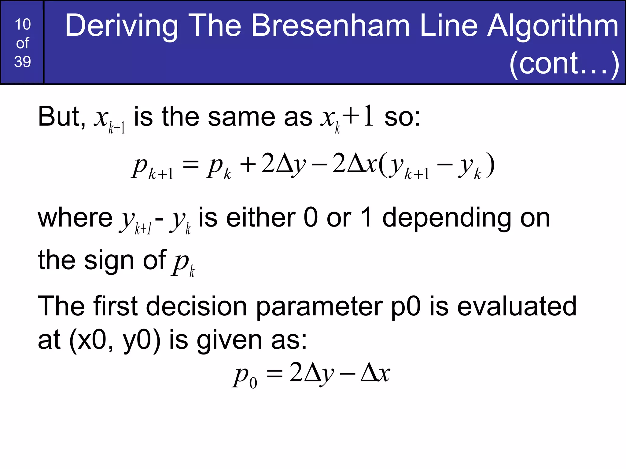
Introduction to Bresenham's algorithm, its advantages using integers, and decision parameters for plotting.
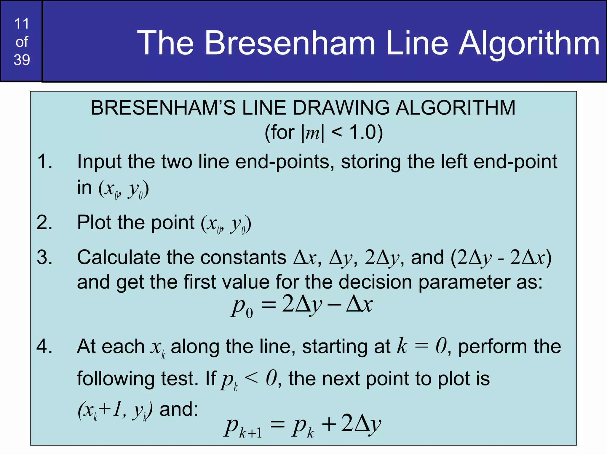
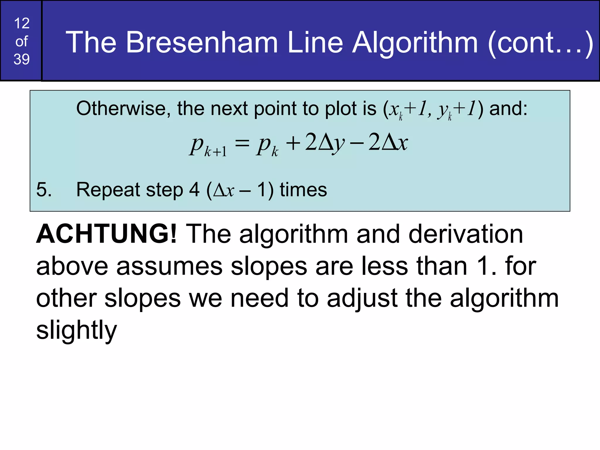
Steps to execute Bresenham's line drawing algorithm tailored for different slopes.
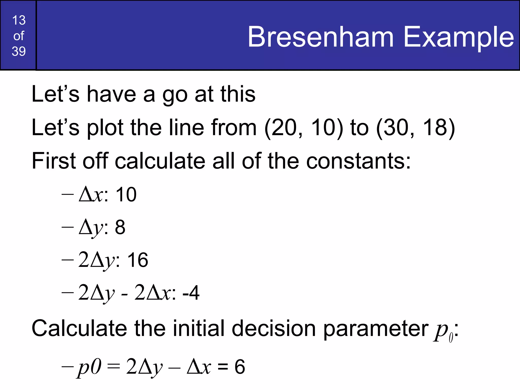
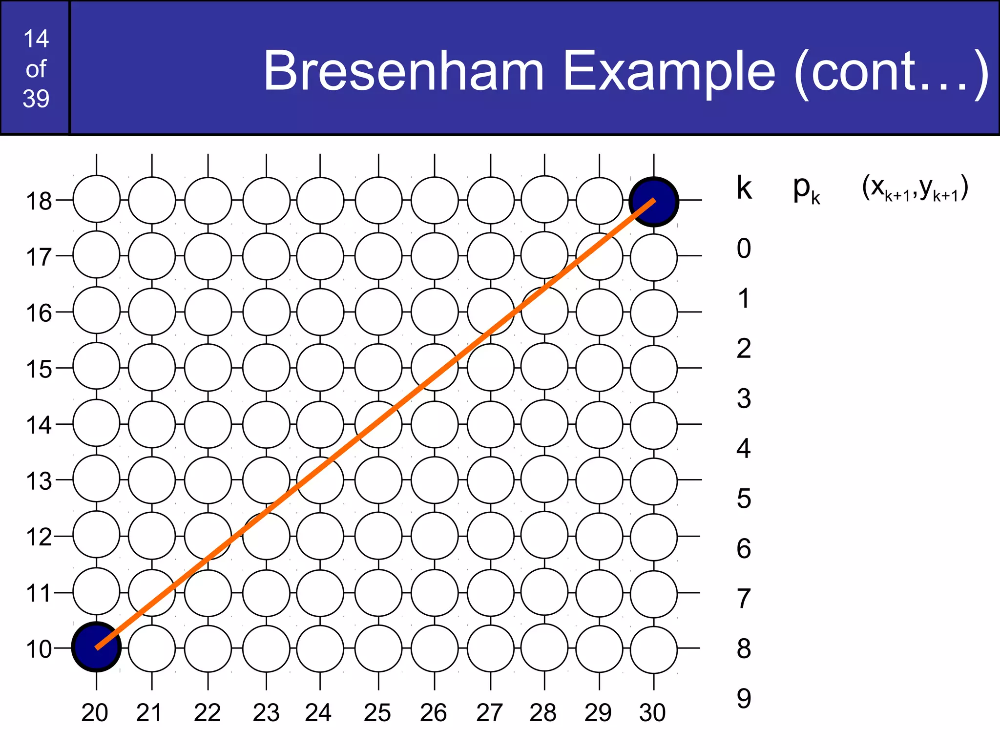
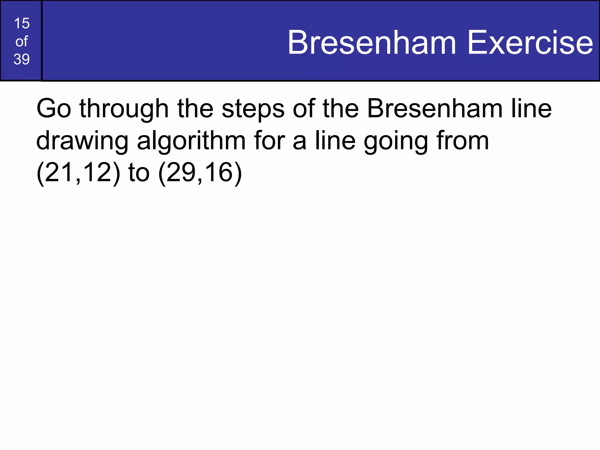
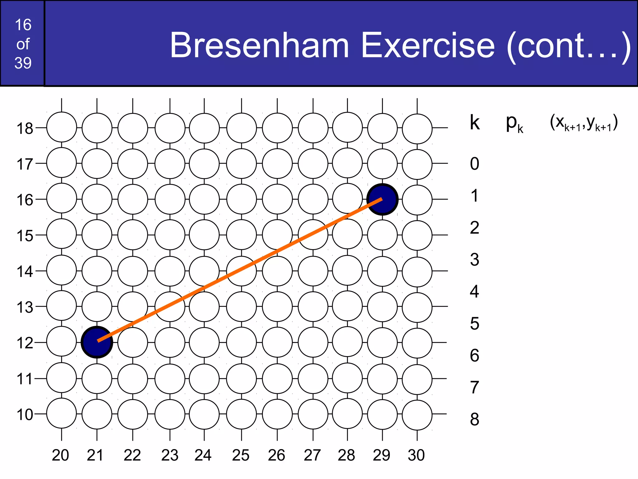
Example application of the algorithm from point (20,10) to (30,18) and an exercise for practice.
Highlights benefits of Bresenham's algorithm over others, specifically highlighting efficiency.
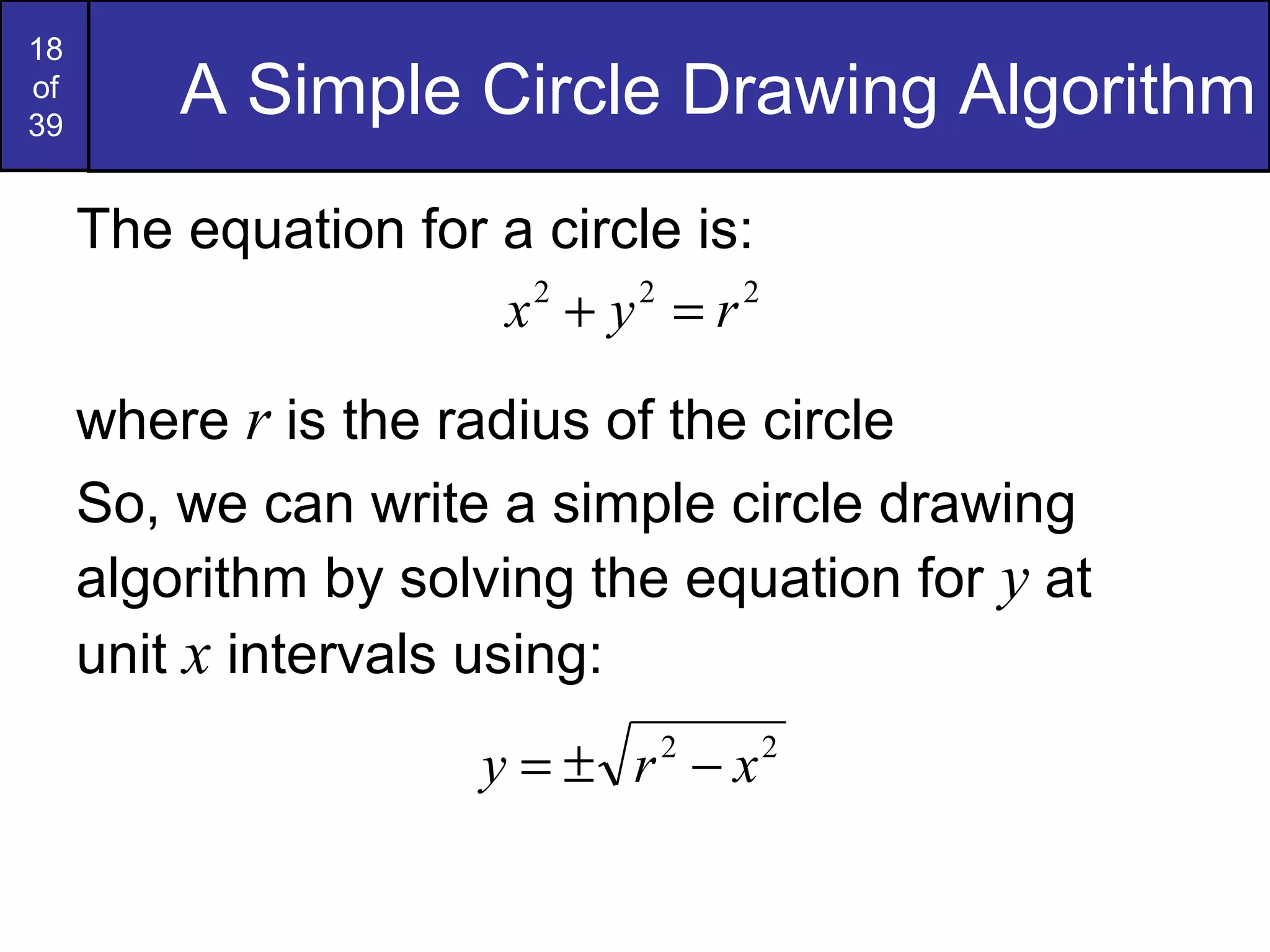
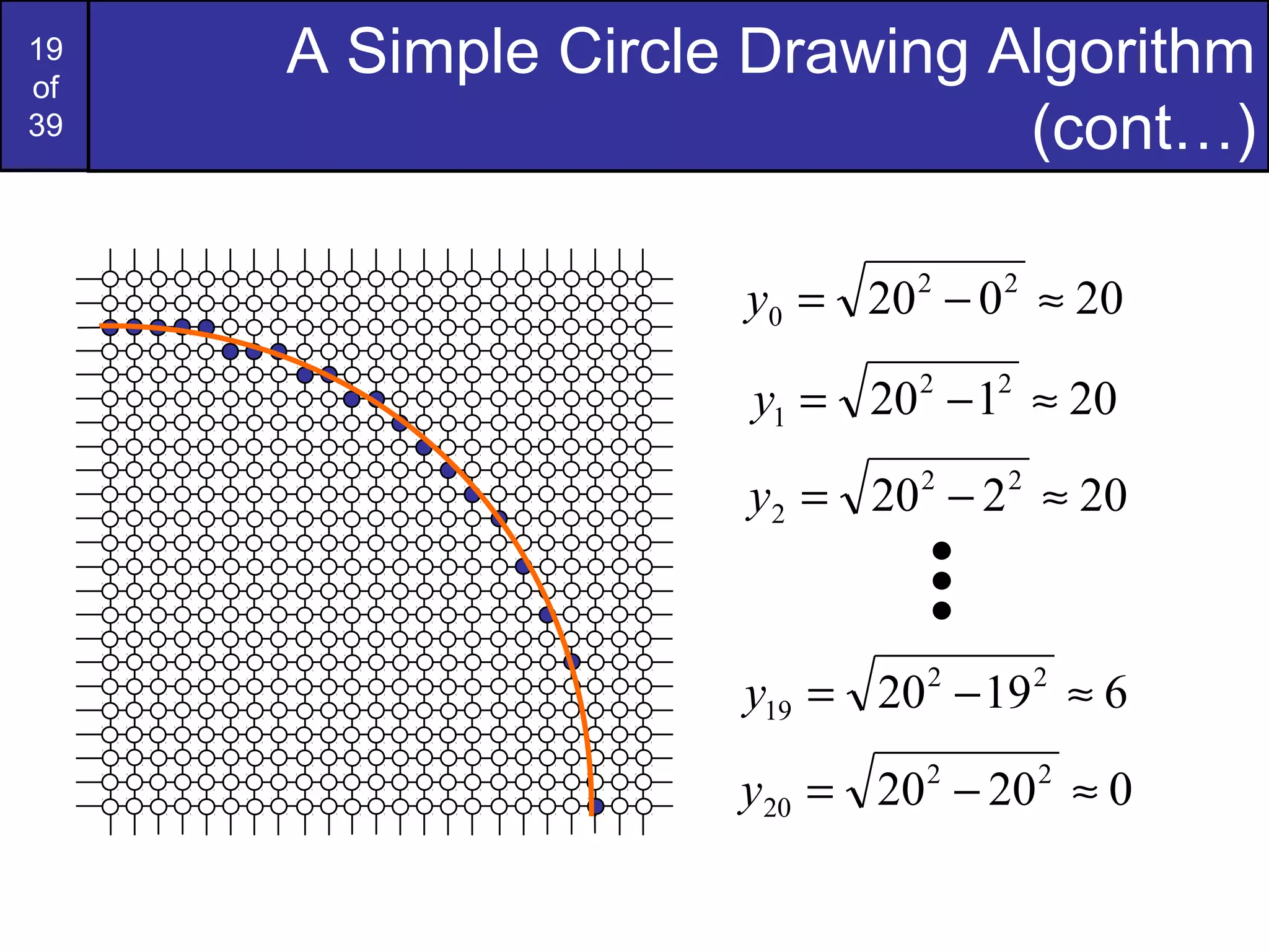
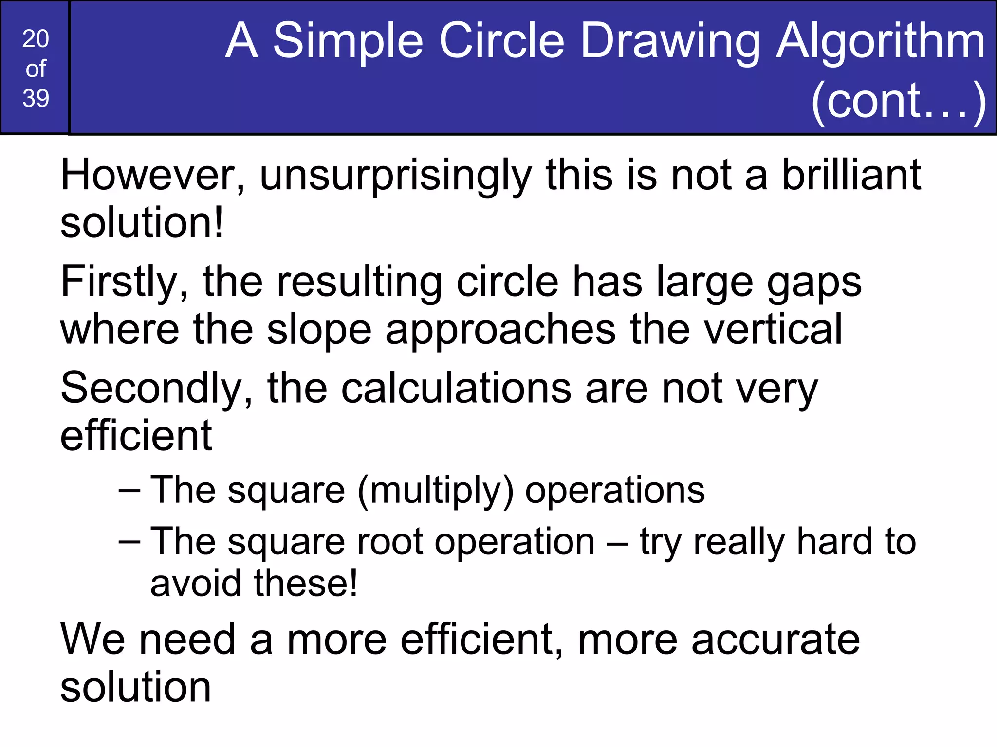
Basic circle drawing algorithm using radius and unit intervals; discusses limitations.
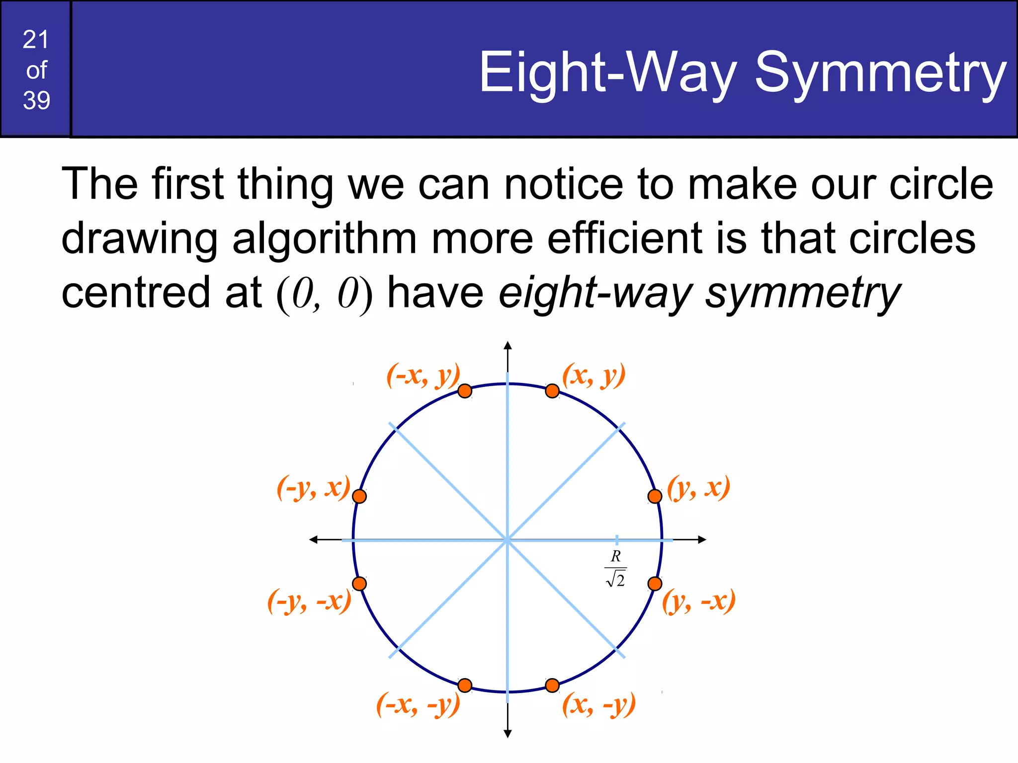
Introduction to the efficiency of using symmetry in circle drawing, including Bresenham's method.
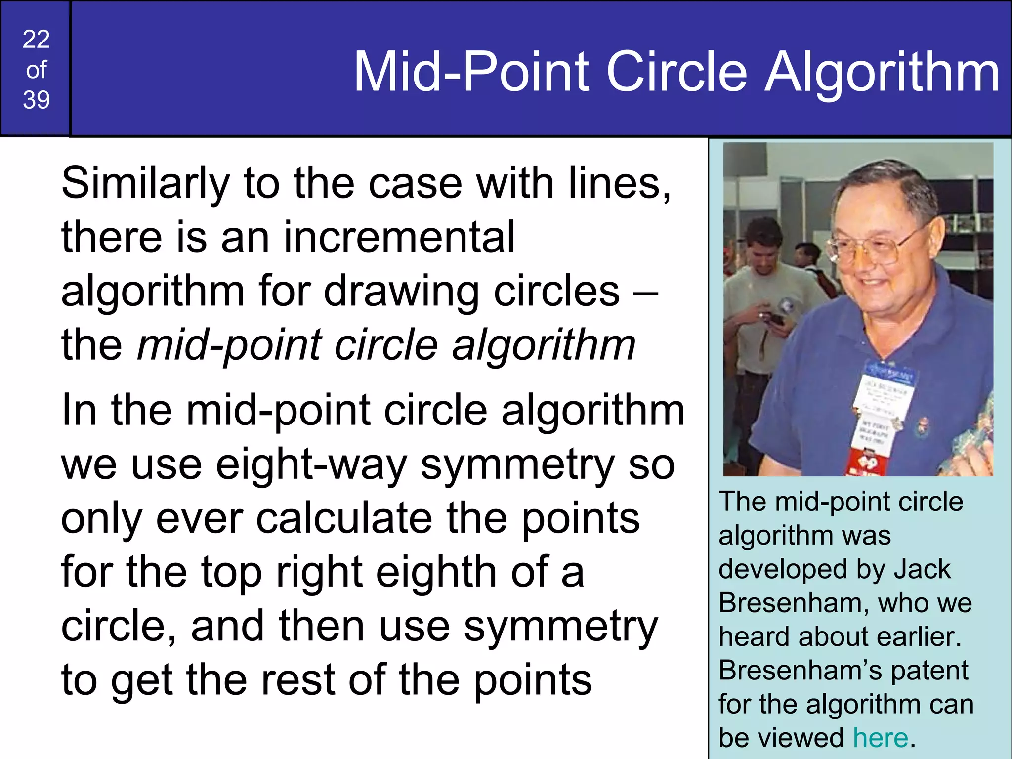
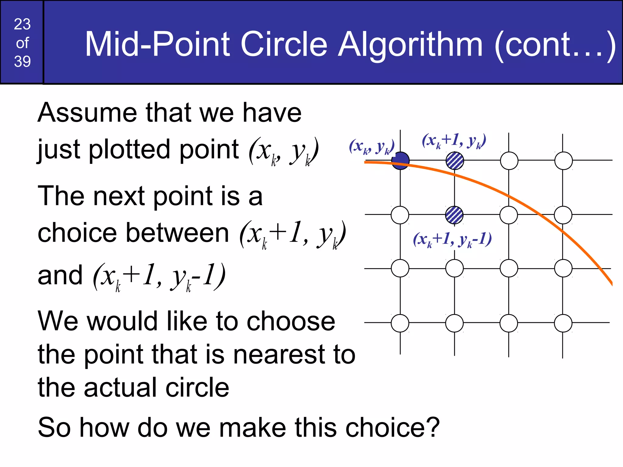
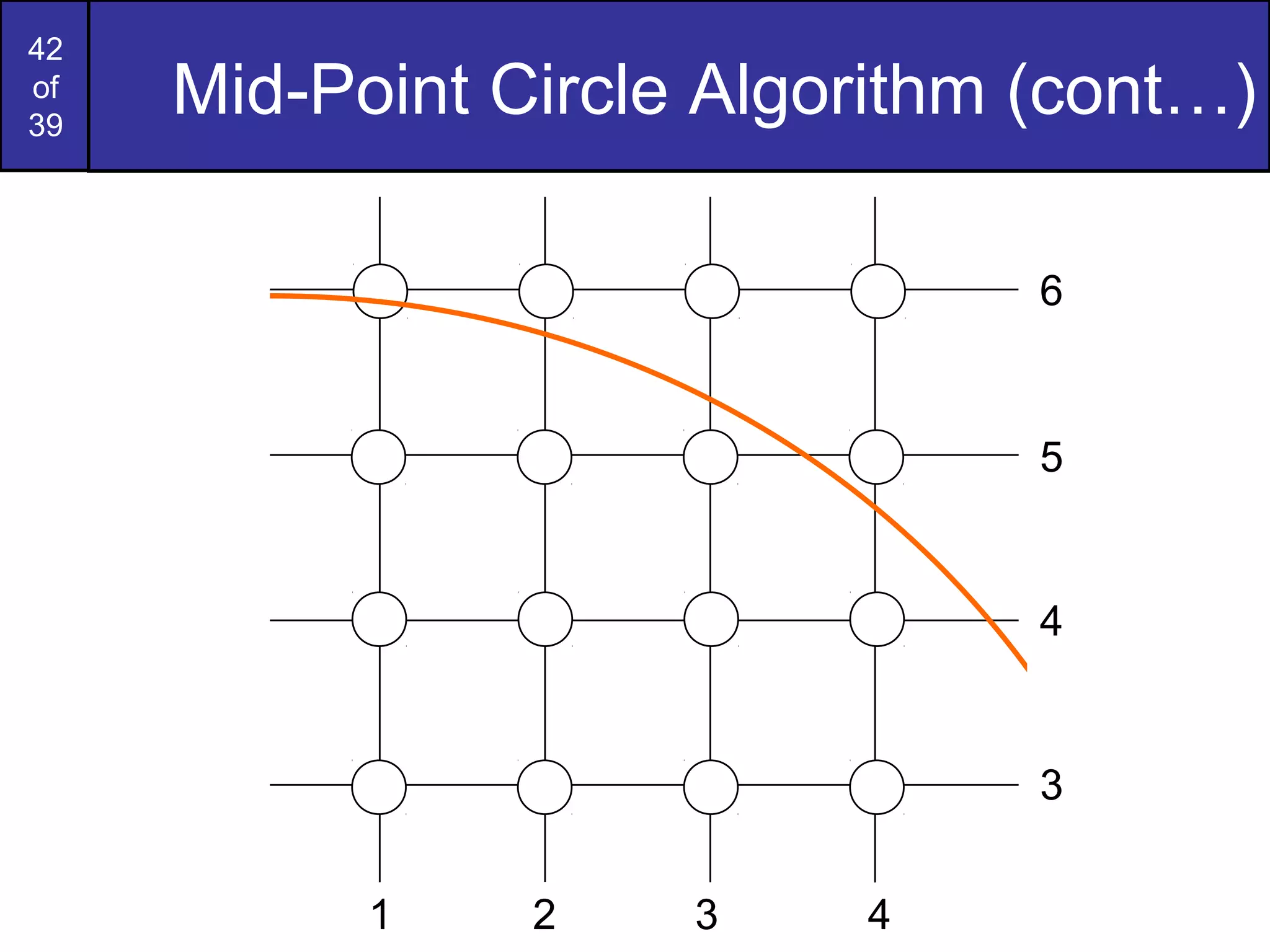
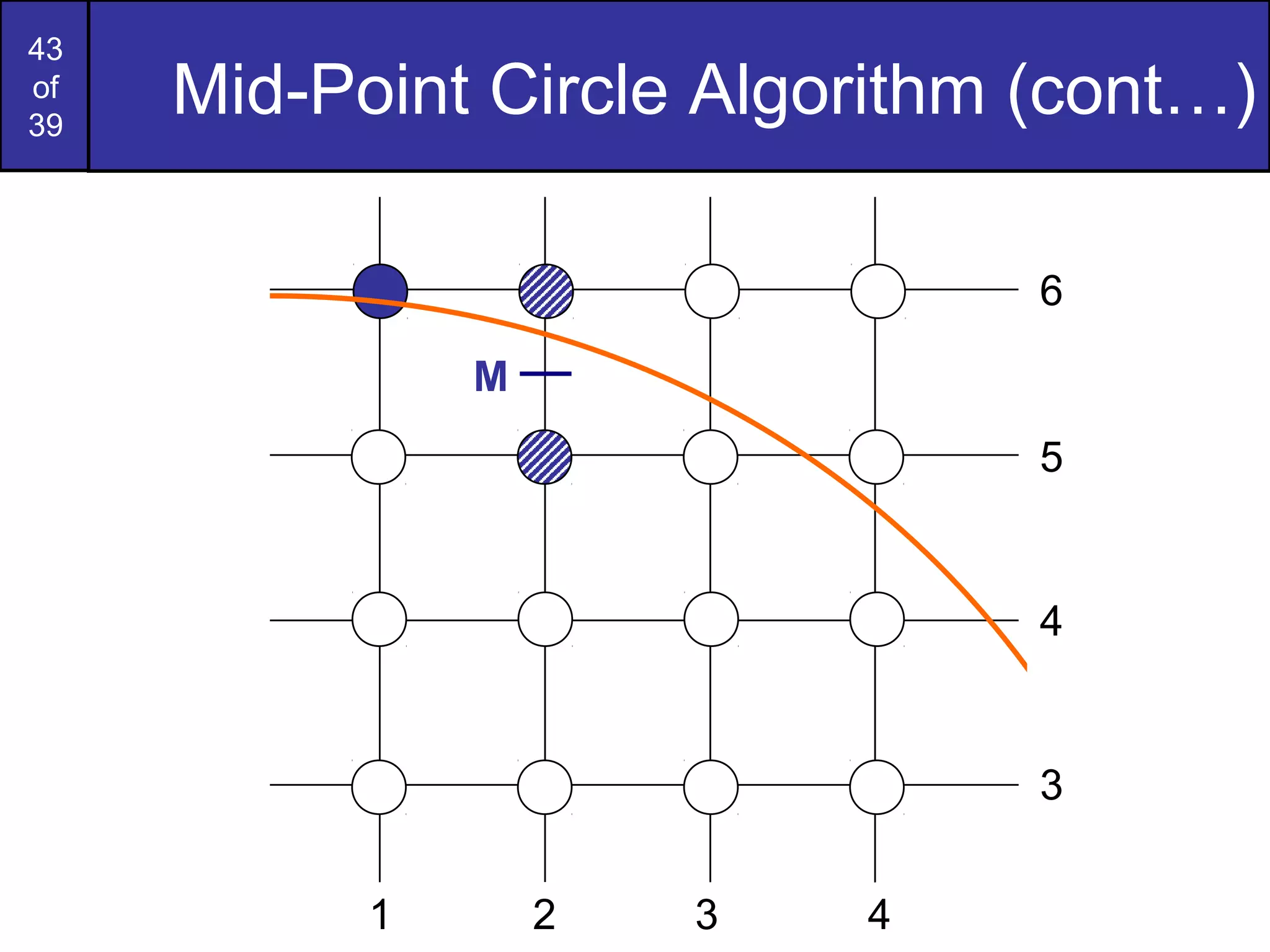
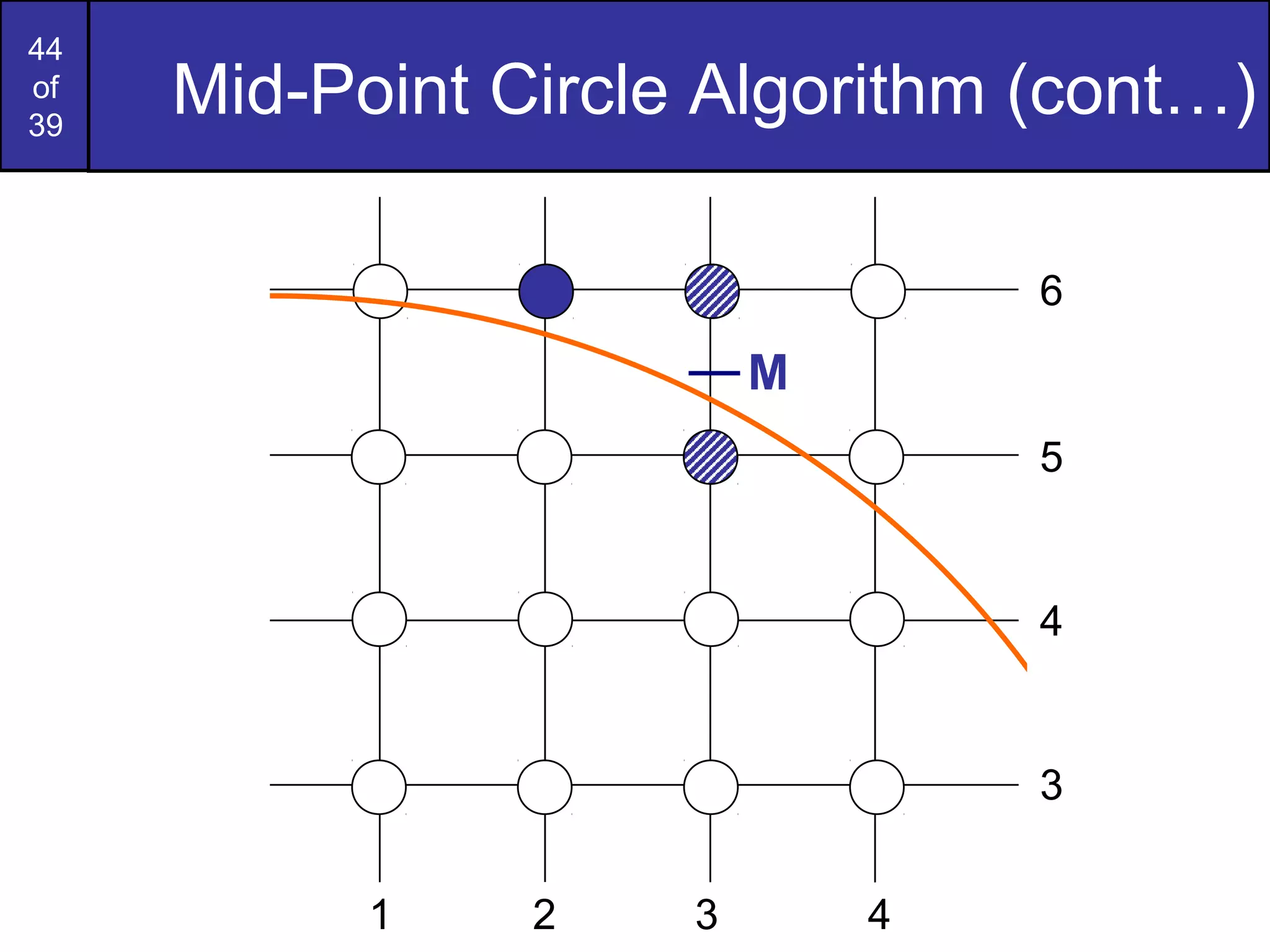
Description and implementation details of the mid-point circle drawing algorithm, incorporating symmetry.
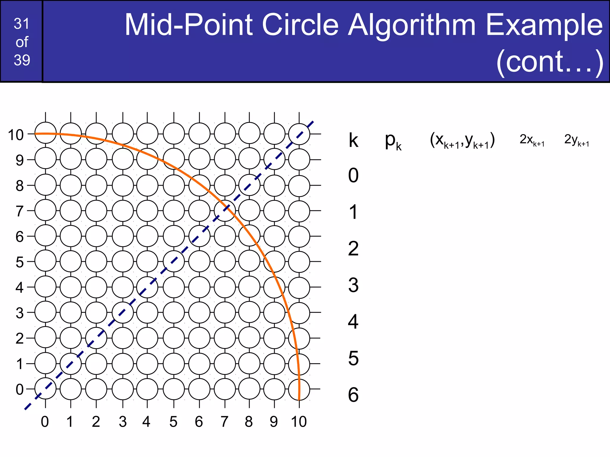
Application of the mid-point algorithm to draw circles, with practice exercises.
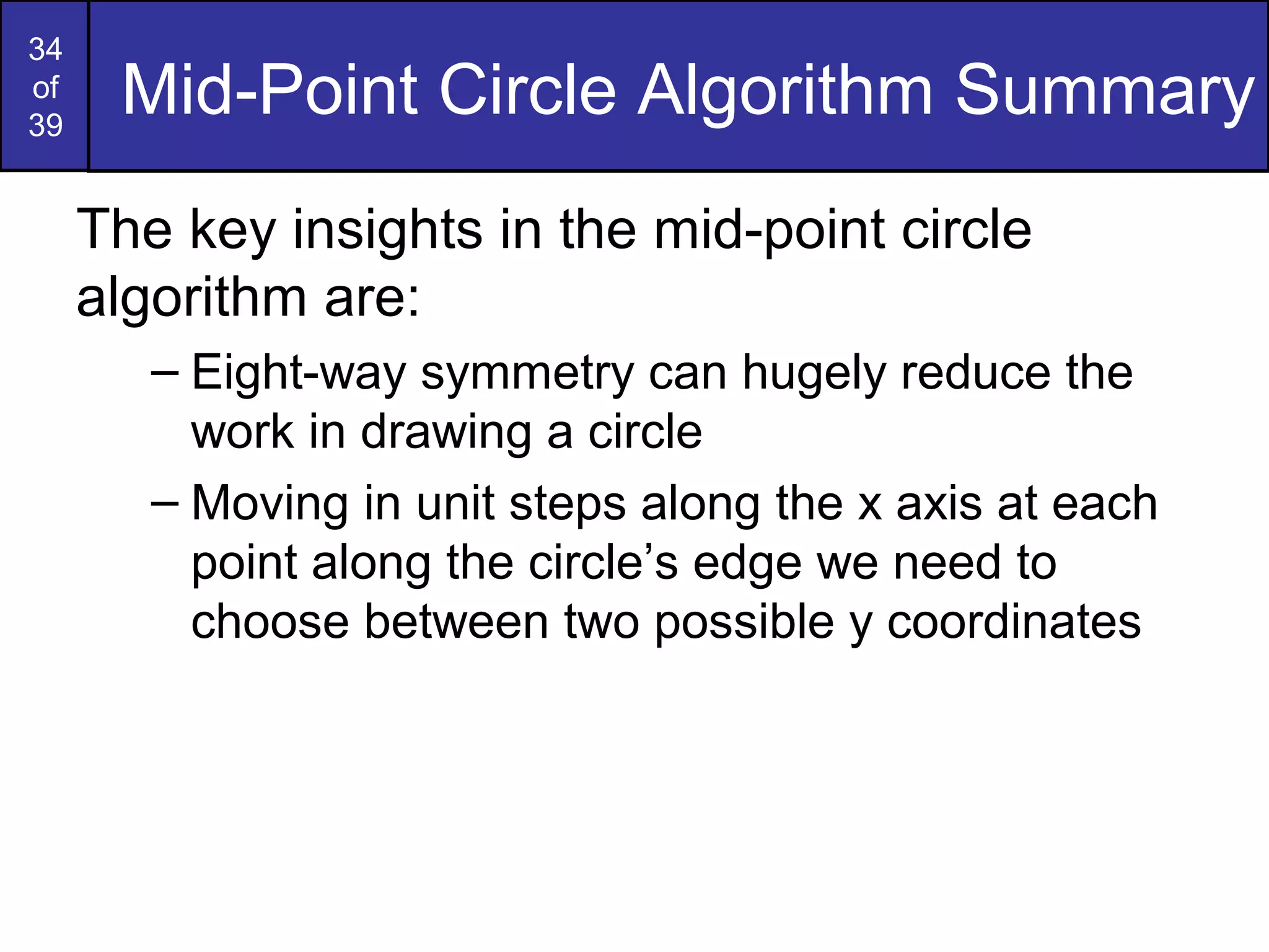
Recap of efficient drawing of circles using symmetry and decision-making along the circumference.
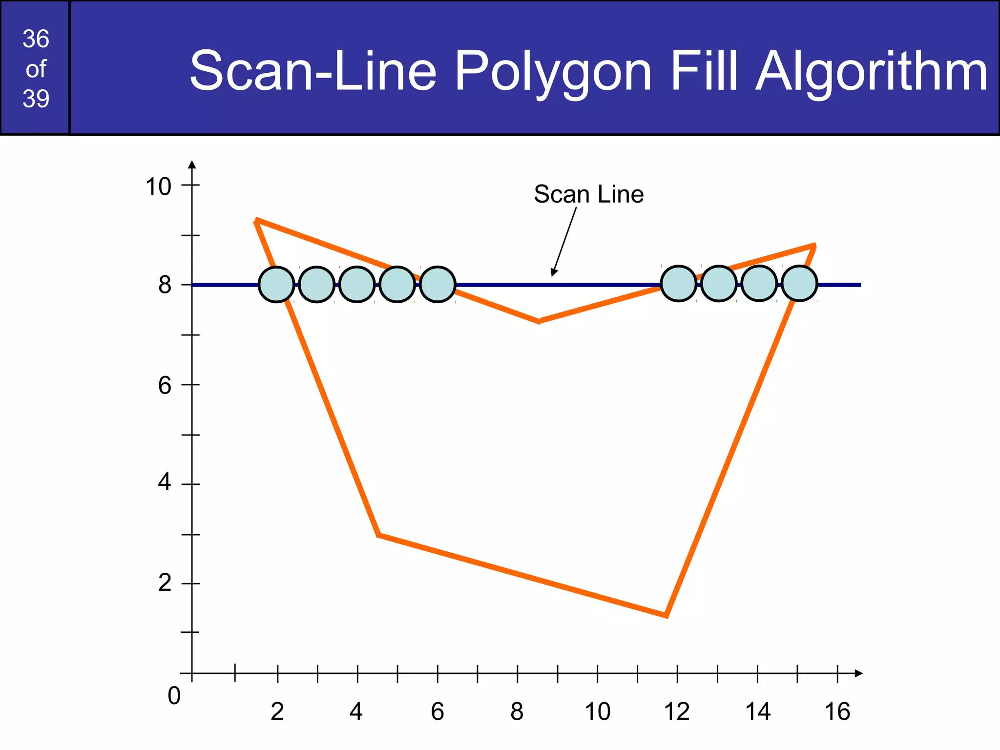
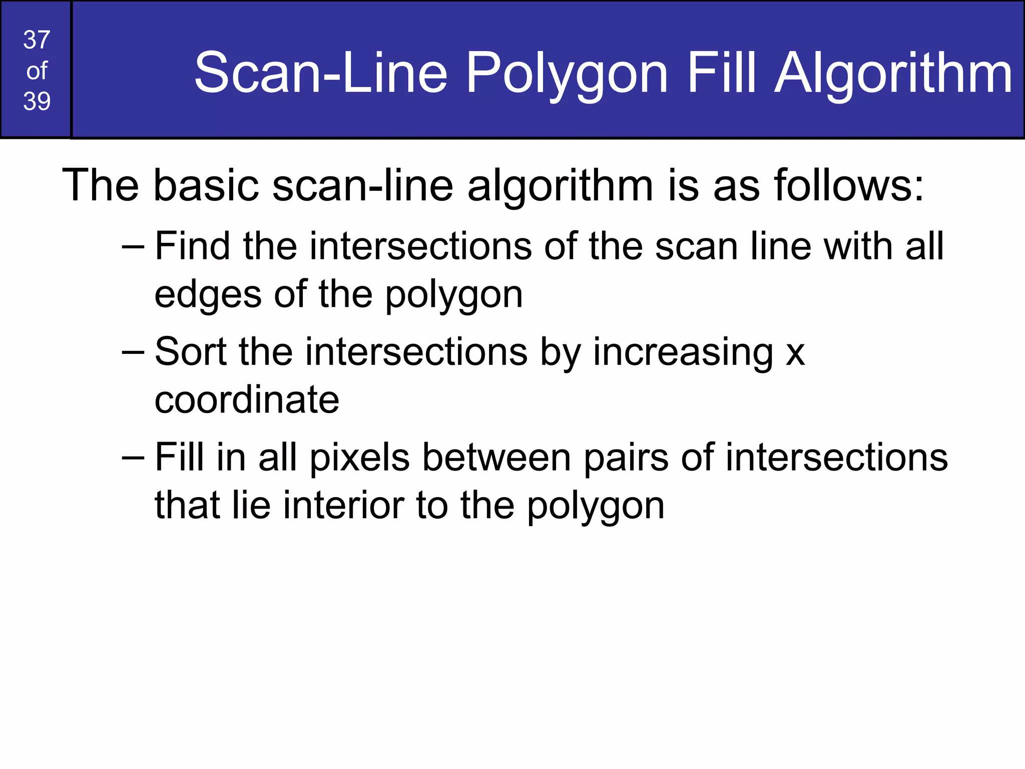
Introduction to the scan-line algorithm for polygon filling, detailing intersection determination.
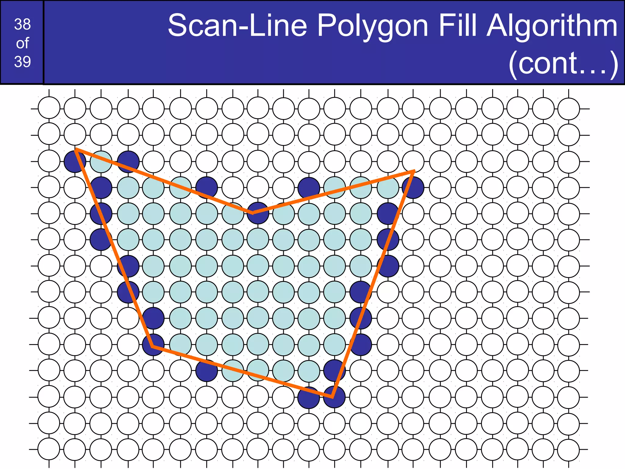
Further exploration of scan-line implementations and filling interiors of polygons.
Summarizes line drawing algorithms discussed, including Bresenham and DDA, emphasizing speed.
Introduction to anti-aliasing techniques in graphics to smooth out jagged edges.
Concluding remarks on various drawing algorithms discussed throughout the presentation.
Additional insights and details related to the mid-point circle algorithm.
Blank grids provided for further practice on drawing algorithms or exercises.


![Chapter 3 - Part 1 [Autosaved].pptx](https://cdn.slidesharecdn.com/ss_thumbnails/chapter3-part1autosaved-230109040832-9344385c-thumbnail.jpg?width=640&height=640&fit=bounds)