Download to read offline
![Innovative Systems Design and Engineering www.iiste.org
ISSN 2222-1727 (Paper) ISSN 2222-2871 (Online)
Vol 3, No 2, 2012
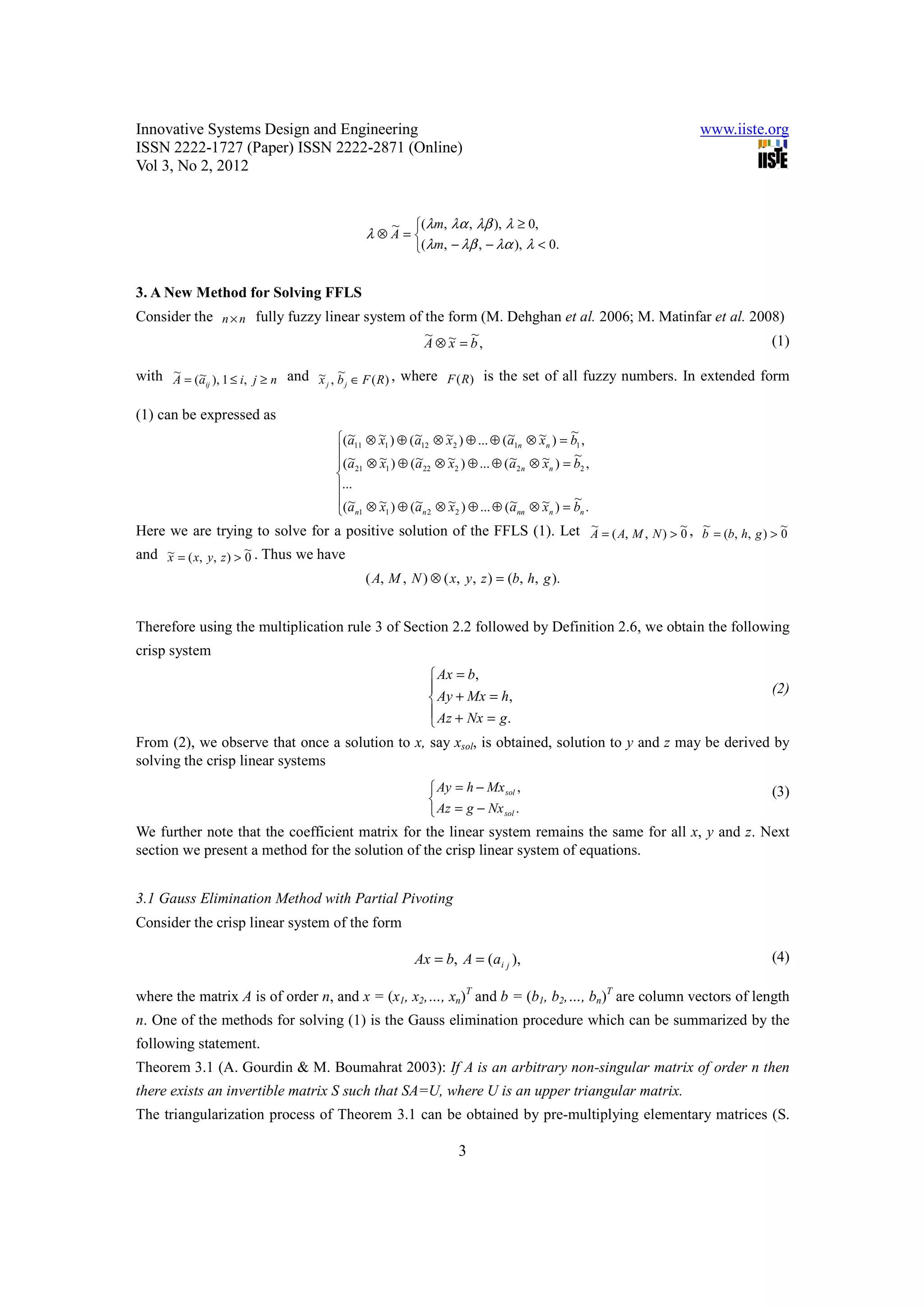
the partial pivoting is introduced. Numerical examples are presented in section 4 to illustrate the method.
2. Preliminaries
In this section, we present some backgrounds and notions of fuzzy sets theory (D. Dubois & H. Prade 1980;
M. Matinfar et al. 2008).
2.1 Definitions
~
Definition 2.1. Assume X to be a universal set, and then a fuzzy subset A of X is defined by its
membership function
µ A : X → [0, 1],
~
where the value of
µ A ( x)
~
~ ~
at x shows the grade of membership of x in A . A fuzzy subset A can be characterized as a set of ordered
µ A ( x)
~
pairs of element x and grade and is often written as
~
A = {( x, µ A ( x )) : x ∈ X }.
~
~
Definition 2.2. A fuzzy set A in X is said to be normal if there exist x ∈ X such that µA(x) =1.
~
~ ~ ~
Definition 2.3. A fuzzy number A is called positive (negative), denoted by A > 0 ( A < 0) , if its membership
function µ A ( x) = 0 ,
~ ∀x < 0 ( x > 0) .
~
Definition 2.4. A triangular fuzzy number, symbolically written as A = (m, α , β ) , has the following
membership function
m − x
1 − α , m − α ≤ x < m , α > 0 ,
x−m
µ A ( x ) = 1 −
~ , m ≤ x ≤ m + β , β > 0,
β
0 , otherwise .
~
Definition 2.5. A triangular fuzzy number A = (m, α , β ) is positive if and only if m − α ≥ 0 .
~ ~
Definition 2.6. Two triangular fuzzy numbers A = (m, α , β ) and B = (n, γ , δ ) are said to be equal if and only
if m = n, α = γ , β = δ .
~
Definition 2.7. A matrix A is called a fuzzy matrix if each of its elements is a fuzzy number. The matrix is
~ ~
positive if each of its elements is positive. The n × n fuzzy matrix A may be represented as A = ( A, M , N ) ,
where A = (aij ) , M = (α ij ) and N = (β i ) are three n × n crisp matrices.
j
2.2 Arithmetic operations on fuzzy numbers
~
In this section, we present arithmetic operations of triangular fuzzy numbers. Let A = (m, α , β ) and
~
B = ( n, γ , δ ) be two triangular fuzzy numbers, then the following rules are valid:
~ ~
1) A ⊕ B = ( m, α , β ) ⊕ (n, γ , δ ) = (m + n, α + γ , β + δ ) .
~
2) − A = −( m, α , β ) = (− m, β , α ) .
~ ~
3) If A > 0 and B > 0 then
~ ~
A ⊗ B = (m, α , β ) ⊗ (n, γ , δ ) = (mn, nα + mγ , nβ + mδ ) .
~
4) If λ is any scalar then λ ⊗ A is defined as
2](https://image.slidesharecdn.com/animplicitpartialpivotinggausseliminationalgorithmforlinearsystemofequationswithfuzzyparameters-120126063715-phpapp01/75/An-implicit-partial-pivoting-gauss-elimination-algorithm-for-linear-system-of-equations-with-fuzzy-parameters-2-2048.jpg)
![Innovative Systems Design and Engineering www.iiste.org
ISSN 2222-1727 (Paper) ISSN 2222-2871 (Online)
Vol 3, No 2, 2012
Lipschutz 2005) (whereby there may be row exchange operations) with the augmented matrix [A | b]. At
each step in the triangularization process, an assumption is made that the term akk is non zero. This term is
called the pivot which is used to eliminate xk from the rows (k + 1) to n. In terms of floating point
arithmetic, dividing by small pivots should be avoided to minimize rounding errors. The partial pivoting is
a well-known strategy to cater for that drawback.
Next we present the Gauss elimination with partial pivoting algorithm where pk is the kth pivot found in the
row lk for k = 1, 2, …, n. We note the algorithm is an implicit approach as there is no exchange of the rows
or columns of the augmented matrix.
Algorithm 3.1: Input – Non-singular matrix A and vector b
Output – Vector x
For k = 1:n - 1,
1. For i = 1:n with i ≠ l1, l2, …, lk-1 select the pivot element pk as pk = max{aik}.
2. For i ≠ l1, l2, …, lk and j = k, k + 1, …, n + 1, triangularize the augmented matrix
by using the formula
a ij = a ij − ( a ik a lk j ) / p k .
3. Solve for x by using the formulae
xn = (alnn+1 ) / pn ,
n
xi = (ali n+1 − ∑a
j =i +1
li j x j ) / pi , i = ( n − 1), ...,1.
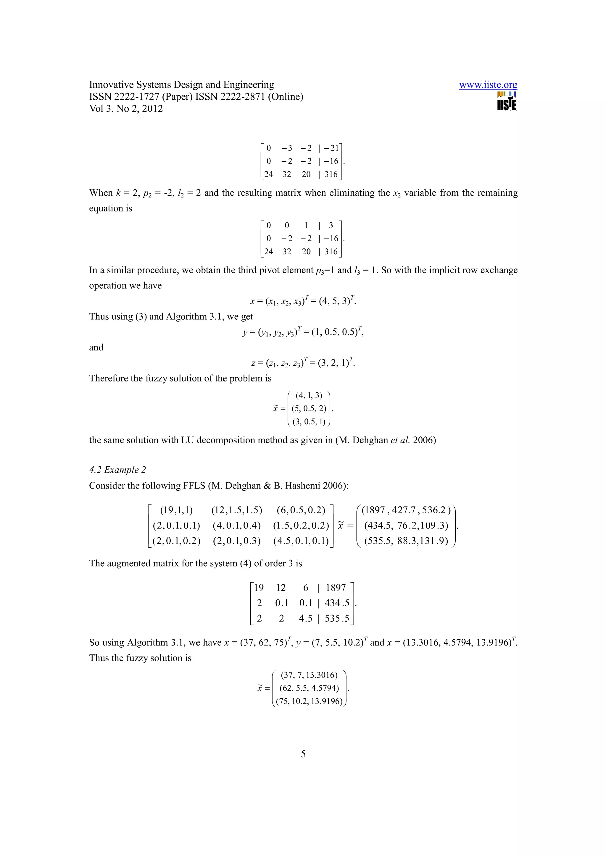
4. Numerical examples
In this section, we apply Algorithm 3.1 for solving fully fuzzy linear system. We implement the algorithm
in the Matlab® software and for the first example we illustrate as well the resulting matrix when eliminating
the xi variable from the remaining equations of the system (3).
4.1 Example 1
Consider the following FFLS (M. Dehghan et al. 2006):
( 6 ,1, 4 ) ( 5, 2 , 2 ) (3, 2, 1) (58 , 30 , 60 )
(12 , 8, 20 )
(14 ,12 , 15 ) (8, 8,10 ) ~ =
x (142, 139, 257) .
( 24 , 10 , 34 ) ( 32 , 30 , 30 )
( 20 , 19 , 24 ) (316, 297, 514)
The augmented matrix for the system (4) of order 3 is
6 5 3 | 58
12 14 8 | 142 .
24
32 20 | 316
Using Algorithm 3.1, we found that when k =1, p1 = 24, l1 = 3 and the resulting matrix when eliminating the
x1 variable from the remaining equations is given as
4](https://image.slidesharecdn.com/animplicitpartialpivotinggausseliminationalgorithmforlinearsystemofequationswithfuzzyparameters-120126063715-phpapp01/75/An-implicit-partial-pivoting-gauss-elimination-algorithm-for-linear-system-of-equations-with-fuzzy-parameters-4-2048.jpg)

![Innovative Systems Design and Engineering www.iiste.org
ISSN 2222-1727 (Paper) ISSN 2222-2871 (Online)
Vol 3, No 2, 2012
the partial pivoting is introduced. Numerical examples are presented in section 4 to illustrate the method.
2. Preliminaries
In this section, we present some backgrounds and notions of fuzzy sets theory (D. Dubois & H. Prade 1980;
M. Matinfar et al. 2008).
2.1 Definitions
~
Definition 2.1. Assume X to be a universal set, and then a fuzzy subset A of X is defined by its
membership function
µ A : X → [0, 1],
~
where the value of
µ A ( x)
~
~ ~
at x shows the grade of membership of x in A . A fuzzy subset A can be characterized as a set of ordered
µ A ( x)
~
pairs of element x and grade and is often written as
~
A = {( x, µ A ( x )) : x ∈ X }.
~
~
Definition 2.2. A fuzzy set A in X is said to be normal if there exist x ∈ X such that µA(x) =1.
~
~ ~ ~
Definition 2.3. A fuzzy number A is called positive (negative), denoted by A > 0 ( A < 0) , if its membership
function µ A ( x) = 0 ,
~ ∀x < 0 ( x > 0) .
~
Definition 2.4. A triangular fuzzy number, symbolically written as A = (m, α , β ) , has the following
membership function
m − x
1 − α , m − α ≤ x < m , α > 0 ,
x−m
µ A ( x ) = 1 −
~ , m ≤ x ≤ m + β , β > 0,
β
0 , otherwise .
~
Definition 2.5. A triangular fuzzy number A = (m, α , β ) is positive if and only if m − α ≥ 0 .
~ ~
Definition 2.6. Two triangular fuzzy numbers A = (m, α , β ) and B = (n, γ , δ ) are said to be equal if and only
if m = n, α = γ , β = δ .
~
Definition 2.7. A matrix A is called a fuzzy matrix if each of its elements is a fuzzy number. The matrix is
~ ~
positive if each of its elements is positive. The n × n fuzzy matrix A may be represented as A = ( A, M , N ) ,
where A = (aij ) , M = (α ij ) and N = (β i ) are three n × n crisp matrices.
j
2.2 Arithmetic operations on fuzzy numbers
~
In this section, we present arithmetic operations of triangular fuzzy numbers. Let A = (m, α , β ) and
~
B = ( n, γ , δ ) be two triangular fuzzy numbers, then the following rules are valid:
~ ~
1) A ⊕ B = ( m, α , β ) ⊕ (n, γ , δ ) = (m + n, α + γ , β + δ ) .
~
2) − A = −( m, α , β ) = (− m, β , α ) .
~ ~
3) If A > 0 and B > 0 then
~ ~
A ⊗ B = (m, α , β ) ⊗ (n, γ , δ ) = (mn, nα + mγ , nβ + mδ ) .
~
4) If λ is any scalar then λ ⊗ A is defined as
2](https://crownmelresort.com/image.slidesharecdn.com/animplicitpartialpivotinggausseliminationalgorithmforlinearsystemofequationswithfuzzyparameters-120126063715-phpapp01/75/An-implicit-partial-pivoting-gauss-elimination-algorithm-for-linear-system-of-equations-with-fuzzy-parameters-2-2048.jpg)

![Innovative Systems Design and Engineering www.iiste.org
ISSN 2222-1727 (Paper) ISSN 2222-2871 (Online)
Vol 3, No 2, 2012
Lipschutz 2005) (whereby there may be row exchange operations) with the augmented matrix [A | b]. At
each step in the triangularization process, an assumption is made that the term akk is non zero. This term is
called the pivot which is used to eliminate xk from the rows (k + 1) to n. In terms of floating point
arithmetic, dividing by small pivots should be avoided to minimize rounding errors. The partial pivoting is
a well-known strategy to cater for that drawback.
Next we present the Gauss elimination with partial pivoting algorithm where pk is the kth pivot found in the
row lk for k = 1, 2, …, n. We note the algorithm is an implicit approach as there is no exchange of the rows
or columns of the augmented matrix.
Algorithm 3.1: Input – Non-singular matrix A and vector b
Output – Vector x
For k = 1:n - 1,
1. For i = 1:n with i ≠ l1, l2, …, lk-1 select the pivot element pk as pk = max{aik}.
2. For i ≠ l1, l2, …, lk and j = k, k + 1, …, n + 1, triangularize the augmented matrix
by using the formula
a ij = a ij − ( a ik a lk j ) / p k .
3. Solve for x by using the formulae
xn = (alnn+1 ) / pn ,
n
xi = (ali n+1 − ∑a
j =i +1
li j x j ) / pi , i = ( n − 1), ...,1.
4. Numerical examples
In this section, we apply Algorithm 3.1 for solving fully fuzzy linear system. We implement the algorithm
in the Matlab® software and for the first example we illustrate as well the resulting matrix when eliminating
the xi variable from the remaining equations of the system (3).
4.1 Example 1
Consider the following FFLS (M. Dehghan et al. 2006):
( 6 ,1, 4 ) ( 5, 2 , 2 ) (3, 2, 1) (58 , 30 , 60 )
(12 , 8, 20 )
(14 ,12 , 15 ) (8, 8,10 ) ~ =
x (142, 139, 257) .
( 24 , 10 , 34 ) ( 32 , 30 , 30 )
( 20 , 19 , 24 ) (316, 297, 514)
The augmented matrix for the system (4) of order 3 is
6 5 3 | 58
12 14 8 | 142 .
24
32 20 | 316
Using Algorithm 3.1, we found that when k =1, p1 = 24, l1 = 3 and the resulting matrix when eliminating the
x1 variable from the remaining equations is given as
4](https://crownmelresort.com/image.slidesharecdn.com/animplicitpartialpivotinggausseliminationalgorithmforlinearsystemofequationswithfuzzyparameters-120126063715-phpapp01/75/An-implicit-partial-pivoting-gauss-elimination-algorithm-for-linear-system-of-equations-with-fuzzy-parameters-4-2048.jpg)


This document proposes a new method for solving fully fuzzy linear systems of equations (FFLS) using Gauss elimination with implicit partial pivoting. It begins by introducing concepts of fuzzy sets theory and arithmetic operations on fuzzy numbers. It then presents the FFLS problem and shows how it can be reduced to a crisp linear system. The key steps of the proposed Gauss elimination method with implicit partial pivoting are outlined. Finally, the method is illustrated on a numerical example, showing the steps to obtain solutions for the variables x, y and z.


![Limits and continuity[1]](https://cdn.slidesharecdn.com/ss_thumbnails/limitsandcontinuity1-110816105053-phpapp01-thumbnail.jpg?width=640&height=640&fit=bounds)