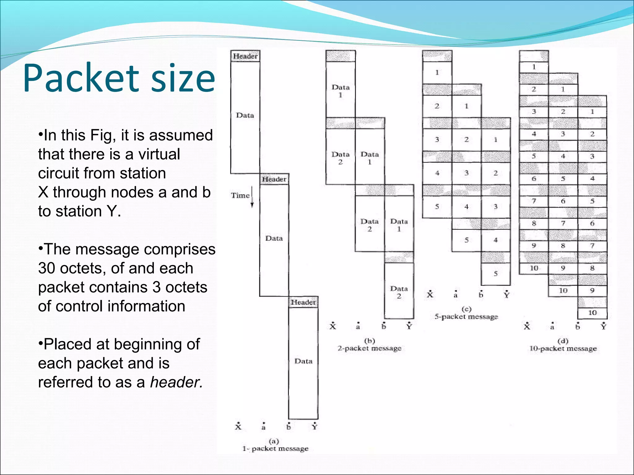
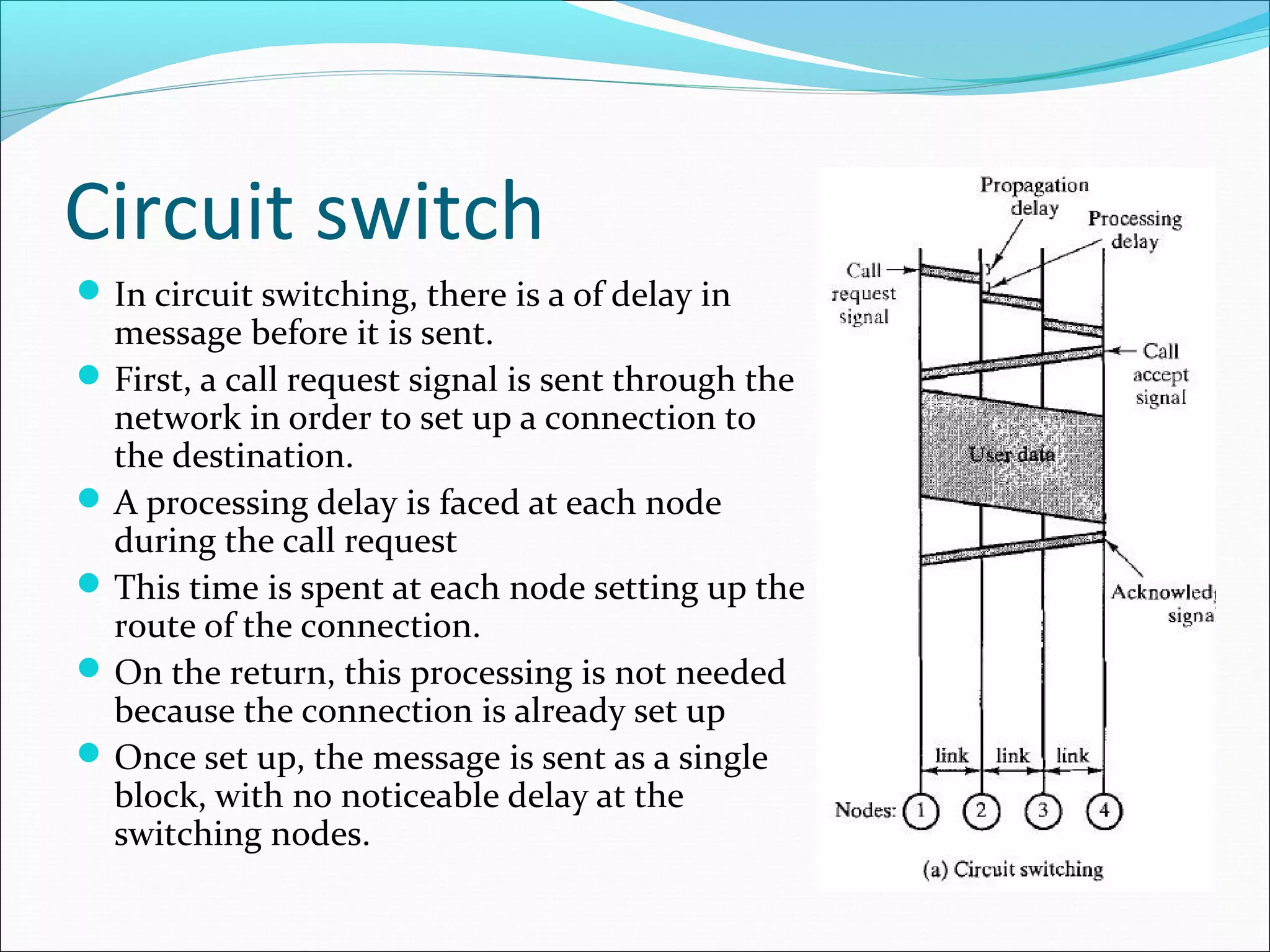
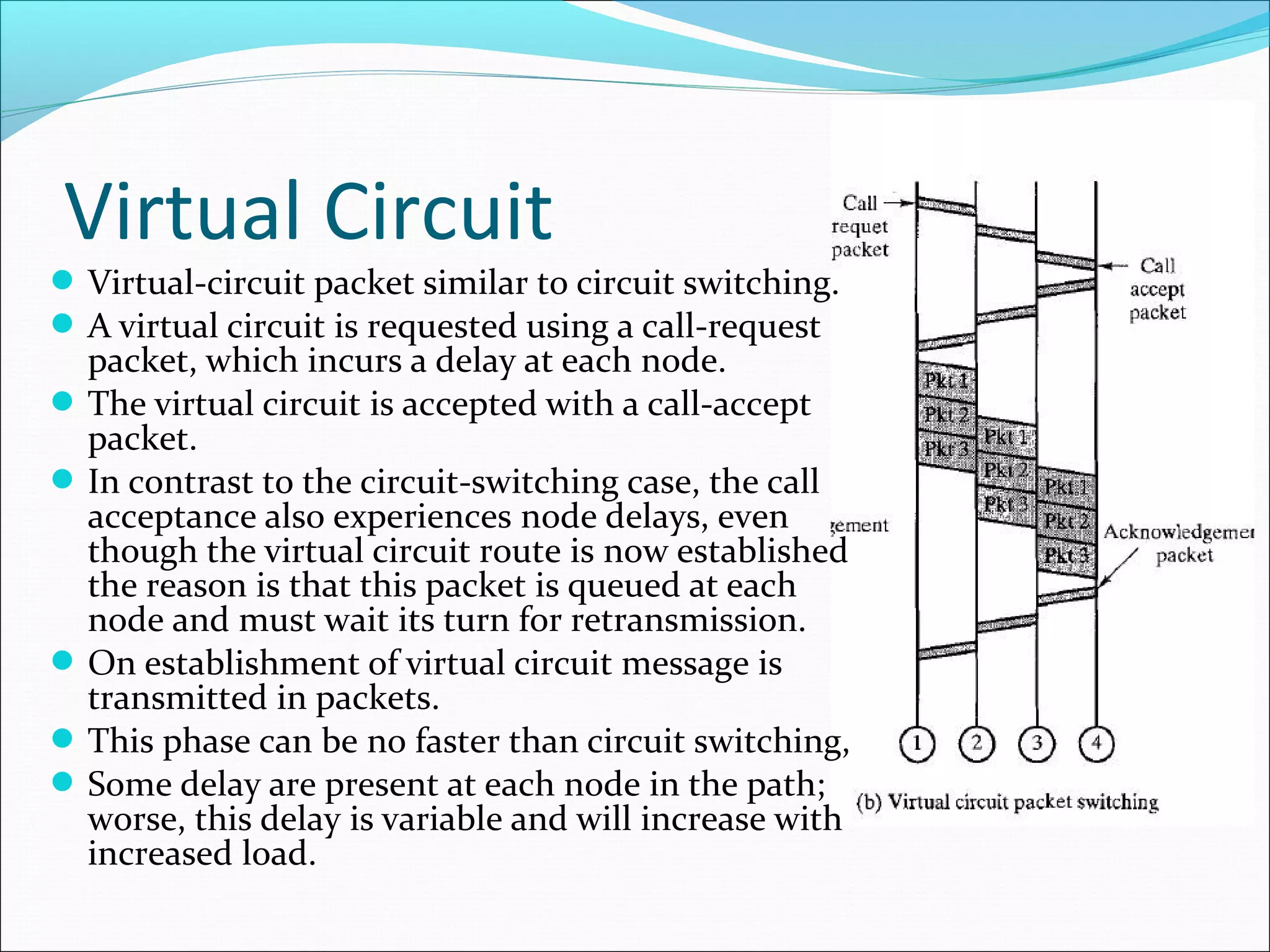
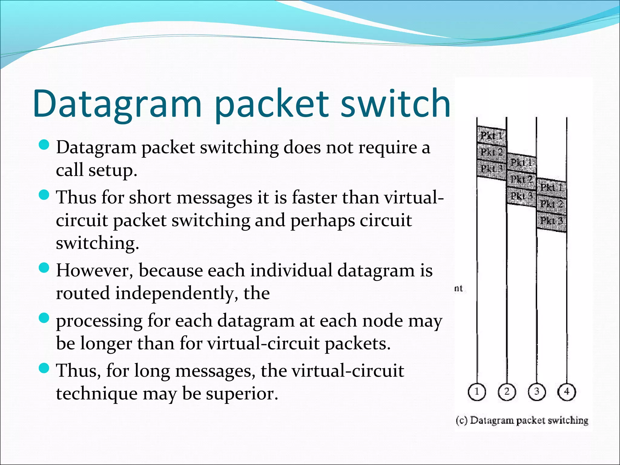
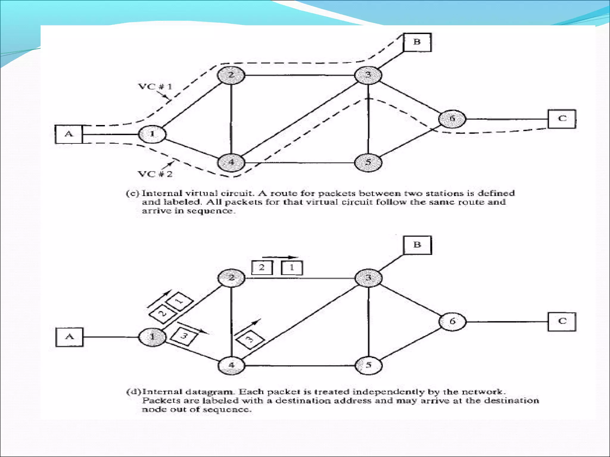
Multiplexing
Introduction
The long-haul circuit-switching telecommunications network was
originally designed to handle voice traffic
A key characteristic of circuit-switching networks is that resources
within the network are dedicated to a particular call. For voice
connections, resulting circuit will enjoy a high percentage of
utilization.
However, as the circuit-switching network began to be used
increasingly for data connections, two shortcomings became
apparent:
 In a typical user host data connection (e.g., personal computer user
logged on to a database server), much of the time the line is idle. Thus,
with data connections, a circuit-switching approach is inefficient.
 In a circuit-switching network, the connection provides for transmission
at constant data rate. Thus, each of the two devices that are connected
must transmit and receive at the same data rate as the other; this limits
the utility of the network in interconnecting a variety of host computers
and terminals.
Solving the problem
To understand how packet switching addresses these
problems, let us briefly summarize packet-switching
operation.
Data are transmitted in short packets. A typical upper
bound on packet length is 1000 octets (bytes).
 If a source has a longer message to send, the message
is broken up into a series of packets
Each packet contains a portion of the user's data plus
some control information.
The control information, at a minimum, includes the
information that the network requires in order to be able
to route the packet through the network
At each node en route, the packet is received, stored
briefly, and passed on to the next node.
The Approach
This approach has a number of advantages over circuit
switching:
Line efficiency is greater, as a single node-to-node link
can be dynamically shared by many packets over time.
The packets are queued up and transmitted as rapidly as
possible over the link.
By contrast, with circuit switching, time on a node-to-
node link is pre-allocated using synchronous TDM.
Much of the time, link may be idle because a portion of
its time is dedicated to a connection which is idle.
Packet-switch network can perform data-rate conversion.
Two stations of different data rates can exchange
packets because each connects to its node at its proper
data rate.
The Approach II
When traffic becomes heavy on a circuit-switching
network, the network refuses to accept additional
connection requests (Blocked) Until load decreases.
On a packet-switching network, packets are still
accepted, but delivery delay increases.
Priorities can be used.
It can transmit the higher-priority packets first. These
packets will therefore experience less delay than
lower-priority packets.
Switching Technique
 A station has a message to send through a packet-switching
network that is of length greater than the maximum packet
size.
 It therefore breaks the message up into packets and sends
these packets, one at a time, to the network.
 A question arises as to how the network will handle this stream
of packets as it attempts to route them through the network
and deliver them to the intended destination
 There are two approaches that are used in contemporary
networks:
 datagram &
 Virtual circuit
Datagram approach
Each packet is treated independently, with no reference to packets
that have gone before.
Some implication of this approach.
When the data is sent over the network it might be possible that the
data packets if broken take different route to its destination
They totally dependent upon the forwarding node for routing the
packets
Possibly the data packet which was last may reach the destination
first.
It is possible for a packet to be destroyed in the network (if a packet
switching node crashes momentarily)
if packets get lost, the destination node has no way to know that one
of the packets in the sequence has been lost.
it is up to receiver to detect loss of a packet and recovers it.
Virtual circuitsIn the virtual-circuit approach, a preplanned route is established
before any packets are sent
It first sends a special control packet, referred to as a Call-Request
packet
Nodes decides to route the request and all subsequent packets to other
nodes
If Station is prepared to accept the connection, it sends Call-Accept
packet back to station via nodes
Stations can then exchange data over the route that has been
established.
As route is fixed for the duration of the logical connection, it is
somewhat similar to a circuit-switching network, and is referred to as
a virtual circuit
Each packet also contains a virtual-circuit identifier and data
Eventually, one of the stations terminates the connection
with a Clear-Request packet
At any time, each station can have more than one virtual circuit to any
other station and can have virtual circuits to more than one station.
Advantages of datagram
In datagram approach the call setup phase is avoided
Datagram delivery will be quicker.
It is more primitive and more flexible
Good with Congestion control-
 Unlike virtual circuits, packets follow a predefined route, it is
difficult to adapt to congestion
Datagram delivery is inherently more reliable
Alternate route that bypasses congestion and failure
A datagram-style of operation is common in inter-
networks
Characteristic of the virtual-circuit
In virtual-circuit (VC) a route between stations is set
up prior to data transfer
That does not mean its a dedicated path
packet is still buffered at each node, and queued for
output over a line
With virtual circuits, the node does not make a
routing decision for transferring each packet
Advantages of VC
If two stations wish to exchange data over an
extended period of time
network may provide services related to the virtual
circuit, including sequencing and error control
because all packets follow the same route, they arrive
in the original order
If dara arrives with an error, node can request a
retransmission of that packet from previous node
Packet size
One important issue is the packet size to be sent on
network
There is a significant relationship between packet size
and transmission time
Packet size
•In this Fig, it is assumed
that there is a virtual
circuit from station
X through nodes a and b
to station Y.
•The message comprises
30 octets, of and each
packet contains 3 octets
of control information
•Placed at beginning of
each packet and is
referred to as a header.
Packet sizeIf the sent packet consists of 33 octets (3 of header plus 30 of data), then
 Packet is first transmitted from station X to node a (Figure a).
 When the entire packet is received, it can then be transmitted from a to b.
 When the entire packet is received at node b, it is transferred to station Y.
 The total transmission time at the nodes is 99 octet-times
(33 octets X 3 packet transmissions = 99 Octet-times).
So if we break up the message into more packets (Packet + Control info)
So because of overlapping in transmission, the total transmission time of 2
packets drops to 72 octet-times, for 5 packets it drop to total of 63
However, this process of using more and smaller packets eventually results
in increased, rather than reduced, delay as in Fig d;
This is because each packet contains a fixed amount of header, and more
packets means more of these headers.
We did not consider processing and queuing delays at each node.
Extremely small packet size (53 octets) can result in an efficient network
design.
Comparison of Circuit Switching
& Packet Switching
Performance
 A simple comparison of circuit switching and the two forms of packet
switching are provided in next slides.
 The figure shows transmission of a message across four nodes. from a
source attached to node 1 to a destination attached to node 4.
In that figure, we are concerned with three types of delay:
 Propagation delay. The time it takes a signal to propagate from one node
to the next. This time is generally negligible in ms
 Transmission time. The time it takes for a transmitter to send out a block
of data. For example, it takes 1 s to transmit a 10,000-bit block of data on a
10-kbps line.
 Node delay. The time it takes for a node to perform the necessary
processing as it switches data.
However, actual performance depends on a host of factors, including
the size of the network, its topology, the pattern of load, and the
characteristics of typical exchanges.
Circuit switch
In circuit switching, there is a of delay in
message before it is sent.
First, a call request signal is sent through the
network in order to set up a connection to
the destination.
A processing delay is faced at each node
during the call request
This time is spent at each node setting up the
route of the connection.
On the return, this processing is not needed
because the connection is already set up
Once set up, the message is sent as a single
block, with no noticeable delay at the
switching nodes.
Virtual Circuit
Virtual-circuit packet similar to circuit switching.
A virtual circuit is requested using a call-request
packet, which incurs a delay at each node.
The virtual circuit is accepted with a call-accept
packet.
In contrast to the circuit-switching case, the call
acceptance also experiences node delays, even
though the virtual circuit route is now established
the reason is that this packet is queued at each
node and must wait its turn for retransmission.
On establishment of virtual circuit message is
transmitted in packets.
This phase can be no faster than circuit switching,
Some delay are present at each node in the path;
worse, this delay is variable and will increase with
increased load.
Datagram packet switching
Datagram packet switching does not require a
call setup.
Thus for short messages it is faster than virtual-
circuit packet switching and perhaps circuit
switching.
However, because each individual datagram is
routed independently, the
processing for each datagram at each node may
be longer than for virtual-circuit packets.
Thus, for long messages, the virtual-circuit
technique may be superior.
Transparency of circuit switching
Circuit switching is essentially a transparent service.
Once a connection is established, a constant data rate is provided to
the connected stations
But not the case with packet switching, which typically introduces
variable
delay, so that data arrive in a choppy manner.
With datagram packet switching, data may arrive in a different order
than they were transmitted.
An additional consequence of transparency is that there is no
overhead required to accommodate circuit switching.
Once a connection is established, the analog or digital data are passed
through, as is, from source to destination.
For packet switching, analog data must be converted to digital before
transmission and each packet includes overhead bits, such as the
destination address.
External and internal operation
Depends upon the characteristics of packet switching
weather it is using data-grams or virtual circuits.
There are two dimensions of these characteristics.
At the interface between a station and network node
Network may provide
 Connection-oriented
 Connectionless service
Connection-oriented service
A station performs a call request to set up a logical connection to
another station
All packets presented to the network are identified as belonging to
a particular logical connection and are numbered sequentially
The logical connection is usually referred to as a virtual circuit and
the connection-oriented service is referred to as an external virtual
circuit service
Where as the external service is distinct from the concept of
internal virtual circuit operation a good example is X.25
X.25 - This standard is almost universally used for interfacing to
packet-switching networks and is employed for packet switching in
ISDN.
Connectionless
With connectionless service, the network only agrees
to handle packets independently, and may not deliver
them in order or reliably, known as an external
datagram service
This concept is distinct from that of internal
datagram operation.
Internally the network may actually construct a fixed
route between endpoints (virtual circuit), or it may
not (datagram).
Design decisions
These internal and external design decisions need not match
External virtual circuit, internal virtual circuit.
 The user requested virtual circuit, a dedicated route through the network.
All packets follow that same route.
External virtual circuit, internal datagram.
 Packets are handled separately. Thus, different packets for the same
external virtual circuit may take different routes. Which are buffered at the
destination node, in proper order.
External datagram, internal datagram.
 Each packet is treated independently from both the user's and the
network's point of view.
External datagram, internal virtual circuit.
 The external user does not see any connections, as it simply sends packets
one at a time. The network, however, sets up a logical connection between
stations for packet delivery and may leave such connections in place for an
extended period, so as to satisfy estimated future needs
Choice
Which one to choose in virtual circuits and data-grams out of both
internal and external.
This will depend on the specific design objectives for the
communication network and the cost factors that prevail.
 The datagram service, allows efficient use of the network as no call setup
and no need to hold up packets while a packet in error is retransmitted.
 This latter feature is desirable in some real-time applications.
 The virtual-circuit service can provide end-to-end sequencing and error
control; this service is attractive for supporting connection-oriented
applications such as file transfer and remote-terminal access.
Virtual-circuit service is much more common than the datagram
service.
The reliability and convenience of a connection-oriented service is
seen as more attractive than the benefits of the datagram service.

8 Packet Switching

  • 1.
  • 2.
    Introduction The long-haul circuit-switchingtelecommunications network was originally designed to handle voice traffic A key characteristic of circuit-switching networks is that resources within the network are dedicated to a particular call. For voice connections, resulting circuit will enjoy a high percentage of utilization. However, as the circuit-switching network began to be used increasingly for data connections, two shortcomings became apparent:  In a typical user host data connection (e.g., personal computer user logged on to a database server), much of the time the line is idle. Thus, with data connections, a circuit-switching approach is inefficient.  In a circuit-switching network, the connection provides for transmission at constant data rate. Thus, each of the two devices that are connected must transmit and receive at the same data rate as the other; this limits the utility of the network in interconnecting a variety of host computers and terminals.
  • 3.
    Solving the problem Tounderstand how packet switching addresses these problems, let us briefly summarize packet-switching operation. Data are transmitted in short packets. A typical upper bound on packet length is 1000 octets (bytes).  If a source has a longer message to send, the message is broken up into a series of packets Each packet contains a portion of the user's data plus some control information. The control information, at a minimum, includes the information that the network requires in order to be able to route the packet through the network At each node en route, the packet is received, stored briefly, and passed on to the next node.
  • 4.
    The Approach This approachhas a number of advantages over circuit switching: Line efficiency is greater, as a single node-to-node link can be dynamically shared by many packets over time. The packets are queued up and transmitted as rapidly as possible over the link. By contrast, with circuit switching, time on a node-to- node link is pre-allocated using synchronous TDM. Much of the time, link may be idle because a portion of its time is dedicated to a connection which is idle. Packet-switch network can perform data-rate conversion. Two stations of different data rates can exchange packets because each connects to its node at its proper data rate.
  • 5.
    The Approach II Whentraffic becomes heavy on a circuit-switching network, the network refuses to accept additional connection requests (Blocked) Until load decreases. On a packet-switching network, packets are still accepted, but delivery delay increases. Priorities can be used. It can transmit the higher-priority packets first. These packets will therefore experience less delay than lower-priority packets.
  • 6.
    Switching Technique  Astation has a message to send through a packet-switching network that is of length greater than the maximum packet size.  It therefore breaks the message up into packets and sends these packets, one at a time, to the network.  A question arises as to how the network will handle this stream of packets as it attempts to route them through the network and deliver them to the intended destination  There are two approaches that are used in contemporary networks:  datagram &  Virtual circuit
  • 7.
    Datagram approach Each packetis treated independently, with no reference to packets that have gone before. Some implication of this approach. When the data is sent over the network it might be possible that the data packets if broken take different route to its destination They totally dependent upon the forwarding node for routing the packets Possibly the data packet which was last may reach the destination first. It is possible for a packet to be destroyed in the network (if a packet switching node crashes momentarily) if packets get lost, the destination node has no way to know that one of the packets in the sequence has been lost. it is up to receiver to detect loss of a packet and recovers it.
  • 8.
    Virtual circuitsIn thevirtual-circuit approach, a preplanned route is established before any packets are sent It first sends a special control packet, referred to as a Call-Request packet Nodes decides to route the request and all subsequent packets to other nodes If Station is prepared to accept the connection, it sends Call-Accept packet back to station via nodes Stations can then exchange data over the route that has been established. As route is fixed for the duration of the logical connection, it is somewhat similar to a circuit-switching network, and is referred to as a virtual circuit Each packet also contains a virtual-circuit identifier and data Eventually, one of the stations terminates the connection with a Clear-Request packet At any time, each station can have more than one virtual circuit to any other station and can have virtual circuits to more than one station.
  • 9.
    Advantages of datagram Indatagram approach the call setup phase is avoided Datagram delivery will be quicker. It is more primitive and more flexible Good with Congestion control-  Unlike virtual circuits, packets follow a predefined route, it is difficult to adapt to congestion Datagram delivery is inherently more reliable Alternate route that bypasses congestion and failure A datagram-style of operation is common in inter- networks
  • 10.
    Characteristic of thevirtual-circuit In virtual-circuit (VC) a route between stations is set up prior to data transfer That does not mean its a dedicated path packet is still buffered at each node, and queued for output over a line With virtual circuits, the node does not make a routing decision for transferring each packet
  • 11.
    Advantages of VC Iftwo stations wish to exchange data over an extended period of time network may provide services related to the virtual circuit, including sequencing and error control because all packets follow the same route, they arrive in the original order If dara arrives with an error, node can request a retransmission of that packet from previous node
  • 12.
    Packet size One importantissue is the packet size to be sent on network There is a significant relationship between packet size and transmission time
  • 13.
    Packet size •In thisFig, it is assumed that there is a virtual circuit from station X through nodes a and b to station Y. •The message comprises 30 octets, of and each packet contains 3 octets of control information •Placed at beginning of each packet and is referred to as a header.
  • 14.
    Packet sizeIf thesent packet consists of 33 octets (3 of header plus 30 of data), then  Packet is first transmitted from station X to node a (Figure a).  When the entire packet is received, it can then be transmitted from a to b.  When the entire packet is received at node b, it is transferred to station Y.  The total transmission time at the nodes is 99 octet-times (33 octets X 3 packet transmissions = 99 Octet-times). So if we break up the message into more packets (Packet + Control info) So because of overlapping in transmission, the total transmission time of 2 packets drops to 72 octet-times, for 5 packets it drop to total of 63 However, this process of using more and smaller packets eventually results in increased, rather than reduced, delay as in Fig d; This is because each packet contains a fixed amount of header, and more packets means more of these headers. We did not consider processing and queuing delays at each node. Extremely small packet size (53 octets) can result in an efficient network design.
  • 15.
    Comparison of CircuitSwitching & Packet Switching Performance  A simple comparison of circuit switching and the two forms of packet switching are provided in next slides.  The figure shows transmission of a message across four nodes. from a source attached to node 1 to a destination attached to node 4. In that figure, we are concerned with three types of delay:  Propagation delay. The time it takes a signal to propagate from one node to the next. This time is generally negligible in ms  Transmission time. The time it takes for a transmitter to send out a block of data. For example, it takes 1 s to transmit a 10,000-bit block of data on a 10-kbps line.  Node delay. The time it takes for a node to perform the necessary processing as it switches data. However, actual performance depends on a host of factors, including the size of the network, its topology, the pattern of load, and the characteristics of typical exchanges.
  • 16.
    Circuit switch In circuitswitching, there is a of delay in message before it is sent. First, a call request signal is sent through the network in order to set up a connection to the destination. A processing delay is faced at each node during the call request This time is spent at each node setting up the route of the connection. On the return, this processing is not needed because the connection is already set up Once set up, the message is sent as a single block, with no noticeable delay at the switching nodes.
  • 17.
    Virtual Circuit Virtual-circuit packetsimilar to circuit switching. A virtual circuit is requested using a call-request packet, which incurs a delay at each node. The virtual circuit is accepted with a call-accept packet. In contrast to the circuit-switching case, the call acceptance also experiences node delays, even though the virtual circuit route is now established the reason is that this packet is queued at each node and must wait its turn for retransmission. On establishment of virtual circuit message is transmitted in packets. This phase can be no faster than circuit switching, Some delay are present at each node in the path; worse, this delay is variable and will increase with increased load.
  • 18.
    Datagram packet switching Datagrampacket switching does not require a call setup. Thus for short messages it is faster than virtual- circuit packet switching and perhaps circuit switching. However, because each individual datagram is routed independently, the processing for each datagram at each node may be longer than for virtual-circuit packets. Thus, for long messages, the virtual-circuit technique may be superior.
  • 19.
    Transparency of circuitswitching Circuit switching is essentially a transparent service. Once a connection is established, a constant data rate is provided to the connected stations But not the case with packet switching, which typically introduces variable delay, so that data arrive in a choppy manner. With datagram packet switching, data may arrive in a different order than they were transmitted. An additional consequence of transparency is that there is no overhead required to accommodate circuit switching. Once a connection is established, the analog or digital data are passed through, as is, from source to destination. For packet switching, analog data must be converted to digital before transmission and each packet includes overhead bits, such as the destination address.
  • 20.
    External and internaloperation Depends upon the characteristics of packet switching weather it is using data-grams or virtual circuits. There are two dimensions of these characteristics. At the interface between a station and network node Network may provide  Connection-oriented  Connectionless service
  • 21.
    Connection-oriented service A stationperforms a call request to set up a logical connection to another station All packets presented to the network are identified as belonging to a particular logical connection and are numbered sequentially The logical connection is usually referred to as a virtual circuit and the connection-oriented service is referred to as an external virtual circuit service Where as the external service is distinct from the concept of internal virtual circuit operation a good example is X.25 X.25 - This standard is almost universally used for interfacing to packet-switching networks and is employed for packet switching in ISDN.
  • 22.
    Connectionless With connectionless service,the network only agrees to handle packets independently, and may not deliver them in order or reliably, known as an external datagram service This concept is distinct from that of internal datagram operation. Internally the network may actually construct a fixed route between endpoints (virtual circuit), or it may not (datagram).
  • 24.
    Design decisions These internaland external design decisions need not match External virtual circuit, internal virtual circuit.  The user requested virtual circuit, a dedicated route through the network. All packets follow that same route. External virtual circuit, internal datagram.  Packets are handled separately. Thus, different packets for the same external virtual circuit may take different routes. Which are buffered at the destination node, in proper order. External datagram, internal datagram.  Each packet is treated independently from both the user's and the network's point of view. External datagram, internal virtual circuit.  The external user does not see any connections, as it simply sends packets one at a time. The network, however, sets up a logical connection between stations for packet delivery and may leave such connections in place for an extended period, so as to satisfy estimated future needs
  • 26.
    Choice Which one tochoose in virtual circuits and data-grams out of both internal and external. This will depend on the specific design objectives for the communication network and the cost factors that prevail.  The datagram service, allows efficient use of the network as no call setup and no need to hold up packets while a packet in error is retransmitted.  This latter feature is desirable in some real-time applications.  The virtual-circuit service can provide end-to-end sequencing and error control; this service is attractive for supporting connection-oriented applications such as file transfer and remote-terminal access. Virtual-circuit service is much more common than the datagram service. The reliability and convenience of a connection-oriented service is seen as more attractive than the benefits of the datagram service.