4-Unconstrained Single Variable Optimization-Methods and Application.pdf
The document discusses unconstrained single variable optimization methods. It covers several topics:
- Direct search methods like bracketing methods, which use only function values, and region elimination methods.
- Methods requiring derivatives like Newton-Raphson, bisection, and secant methods, which use function and derivative values.
- Specific methods covered in more detail include exhaustive search, bounding phase, dichotomous search, and interval halving for region elimination. Algorithms for some of these methods are provided.
4-Unconstrained Single Variable Optimization-Methods and Application.pdf
1.
ChE – 422PROCESS ANALYSIS & OPTIMIZATION
Unconstrained Single Variable Optimization
(Methods and Application )
Saeed GUL, Professor
Department of Chemical Engineering,
University of Engineering & Technology Peshawar, PAKISTAN
2.
Unconstrained single variableoptimization
18 January
2022
Department of Chemical Engineering, UET Peshawar, Pakistan 2
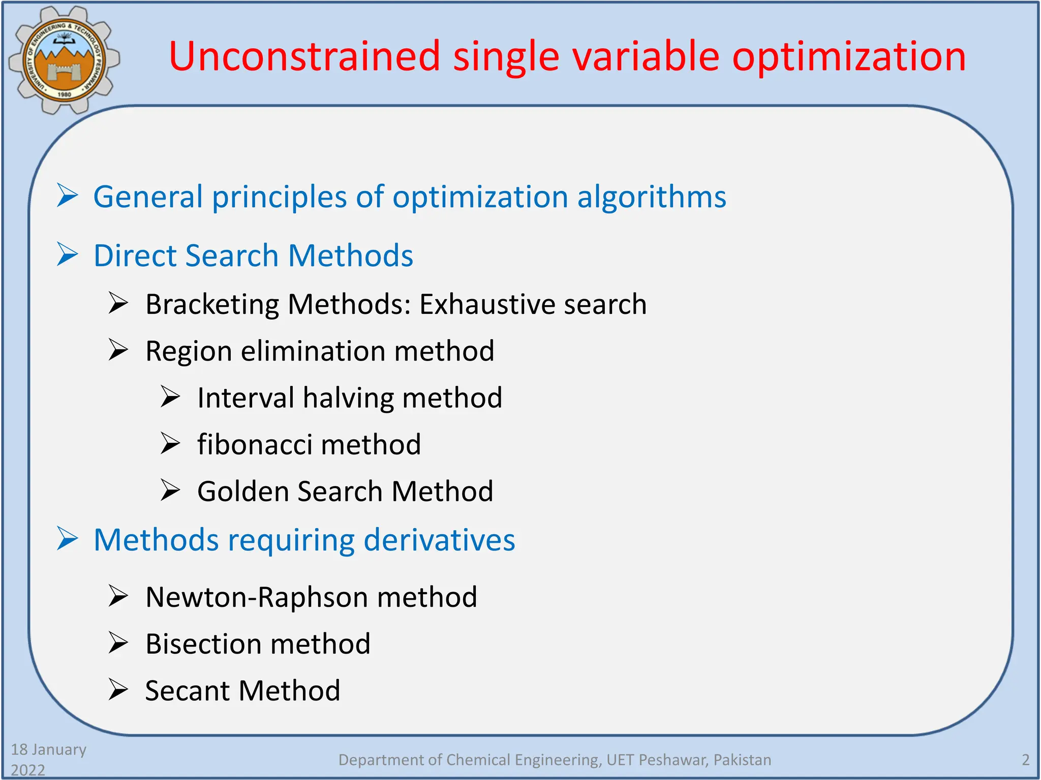
General principles of optimization algorithms
Direct Search Methods
Bracketing Methods: Exhaustive search
Region elimination method
Interval halving method
fibonacci method
Golden Search Method
Methods requiring derivatives
Newton-Raphson method
Bisection method
Secant Method
3.
Unconstrained single variableoptimization
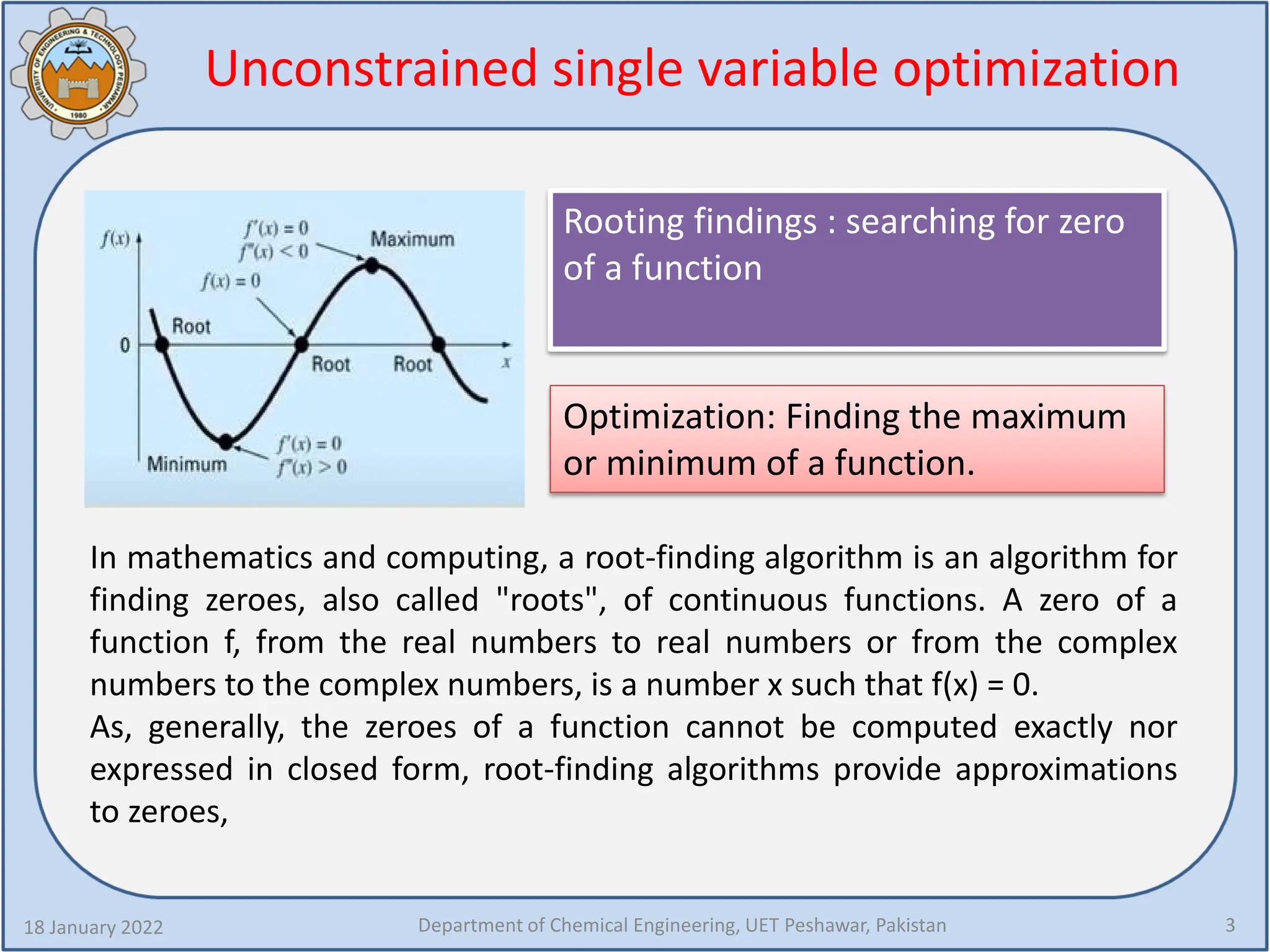
Rooting findings : searching for zero
of a function
18 January 2022 Department of Chemical Engineering, UET Peshawar, Pakistan 3
Optimization: Finding the maximum
or minimum of a function.
In mathematics and computing, a root-finding algorithm is an algorithm for
finding zeroes, also called "roots", of continuous functions. A zero of a
function f, from the real numbers to real numbers or from the complex
numbers to the complex numbers, is a number x such that f(x) = 0.
As, generally, the zeroes of a function cannot be computed exactly nor
expressed in closed form, root-finding algorithms provide approximations
to zeroes,
4.
Unconstrained single variableoptimization
problems:
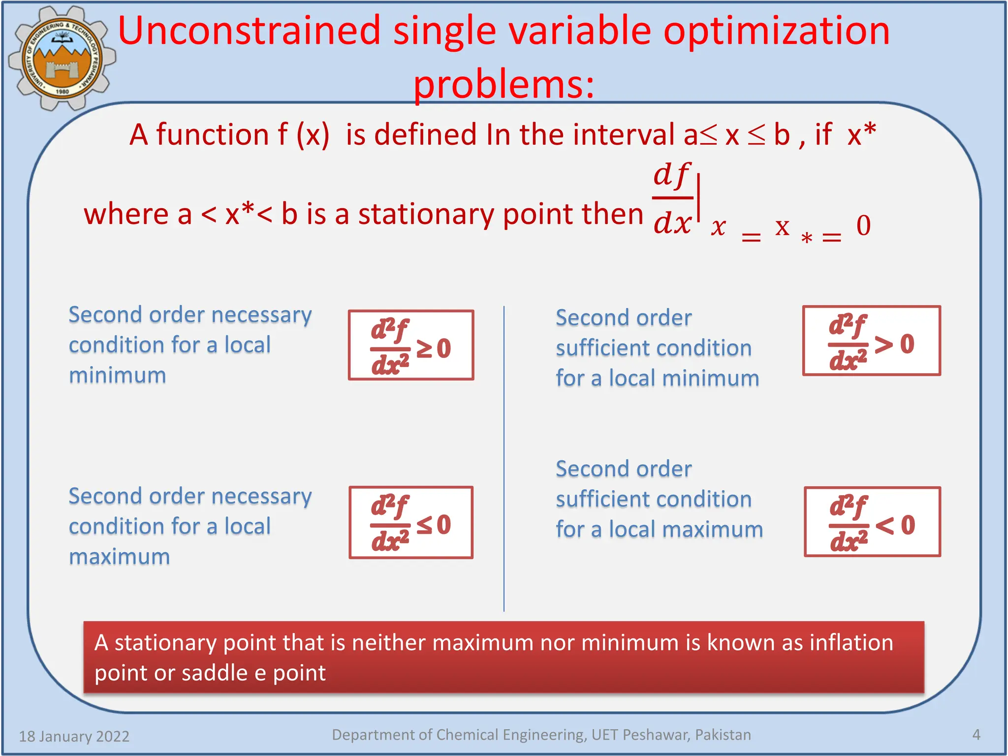
A function f (x) is defined In the interval a≤ x ≤ b , if x*
where a < x*< b is a stationary point then
𝑑𝑑𝑑𝑑
𝑑𝑑𝑑𝑑
�
𝑥𝑥 = x ∗ = 0
18 January 2022 Department of Chemical Engineering, UET Peshawar, Pakistan 4
Second order necessary
condition for a local
minimum
Second order necessary
condition for a local
maximum
Second order
sufficient condition
for a local minimum
Second order
sufficient condition
for a local maximum
A stationary point that is neither maximum nor minimum is known as inflation
point or saddle e point
5.
Unconstrained single variableoptimization
problems:
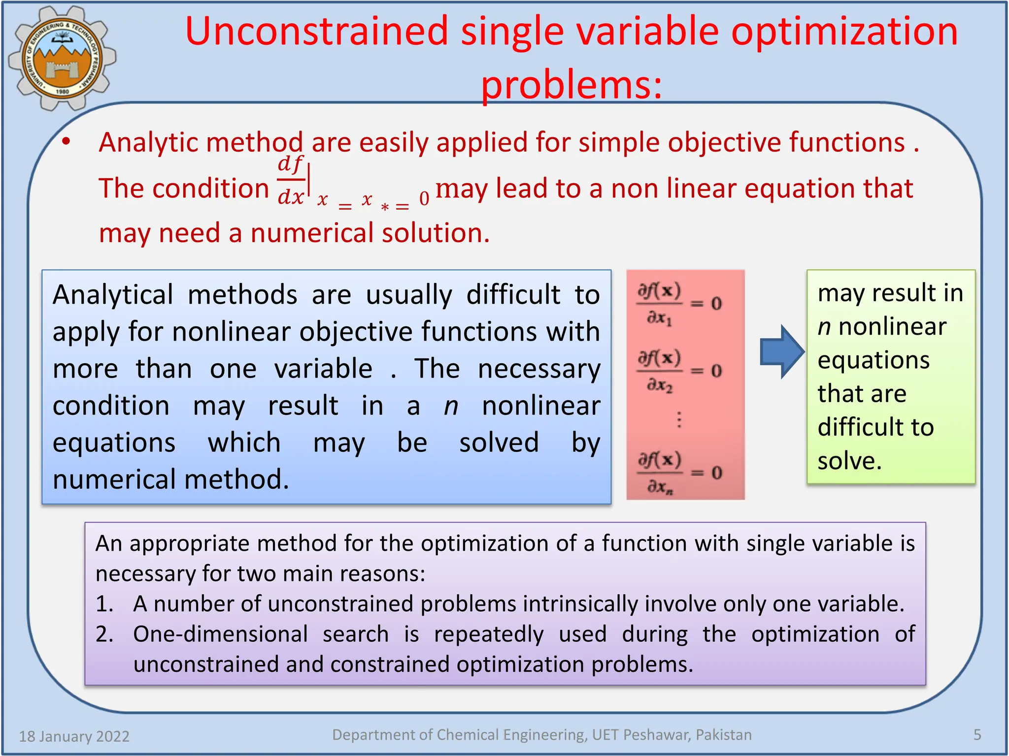
• Analytic method are easily applied for simple objective functions .
The condition
𝑑𝑑𝑑𝑑
𝑑𝑑𝑑𝑑
�
𝑥𝑥 = 𝑥𝑥 ∗ = 0 may lead to a non linear equation that
may need a numerical solution.
18 January 2022 Department of Chemical Engineering, UET Peshawar, Pakistan 5
Analytical methods are usually difficult to
apply for nonlinear objective functions with
more than one variable . The necessary
condition may result in a n nonlinear
equations which may be solved by
numerical method.
may result in
n nonlinear
equations
that are
difficult to
solve.
An appropriate method for the optimization of a function with single variable is
necessary for two main reasons:
1. A number of unconstrained problems intrinsically involve only one variable.
2. One-dimensional search is repeatedly used during the optimization of
unconstrained and constrained optimization problems.
6.
A general optimizationalgorithm
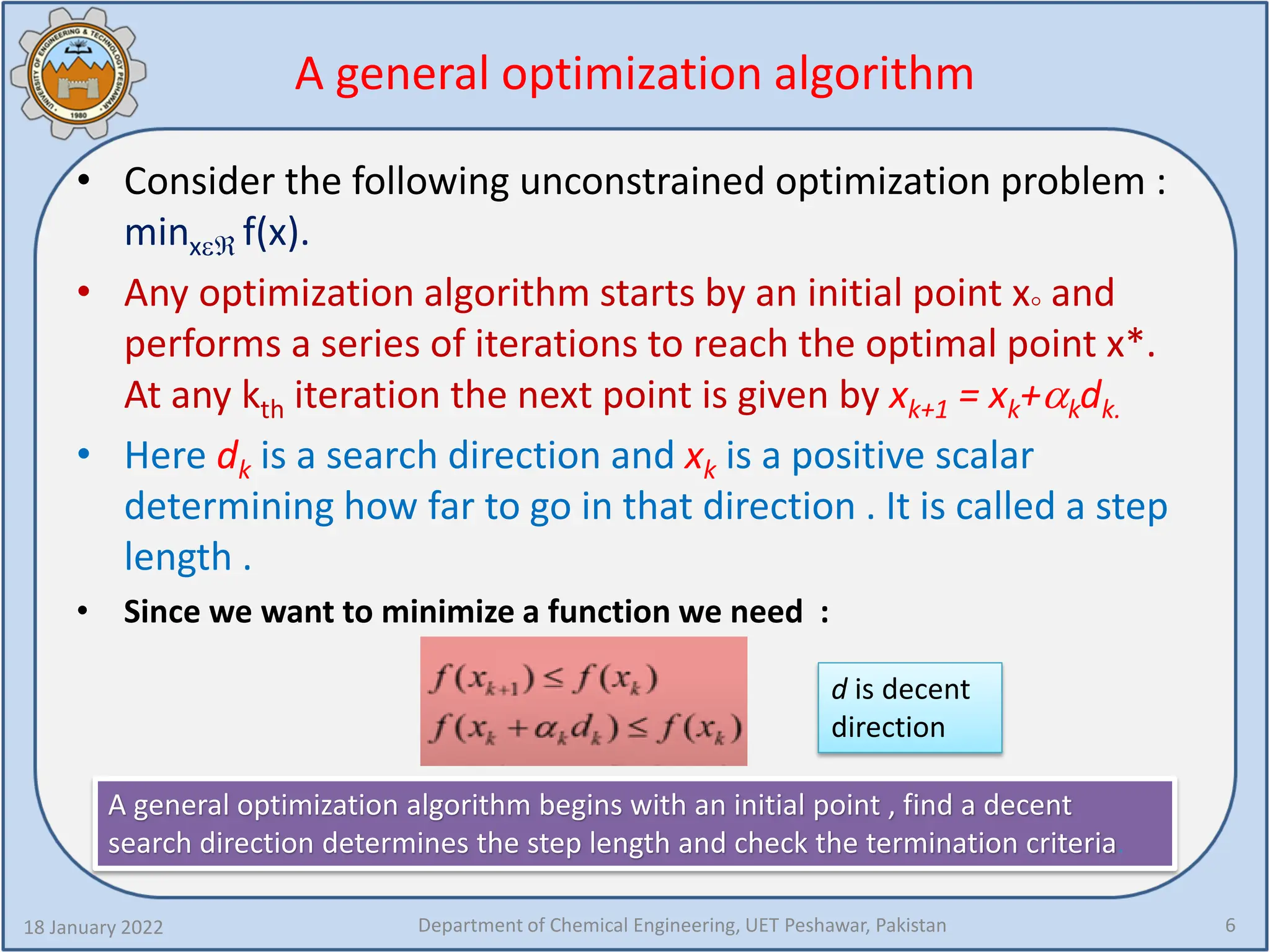
• Consider the following unconstrained optimization problem :
minxεℜ f(x).
• Any optimization algorithm starts by an initial point x° and
performs a series of iterations to reach the optimal point x*.
At any kth iteration the next point is given by xk+1 = xk+αkdk.
• Here dk is a search direction and xk is a positive scalar
determining how far to go in that direction . It is called a step
length .
• Since we want to minimize a function we need :
18 January 2022 Department of Chemical Engineering, UET Peshawar, Pakistan 6
d is decent
direction
A general optimization algorithm begins with an initial point , find a decent
search direction determines the step length and check the termination criteria.
7.
A general optimizationalgorithm cont,d
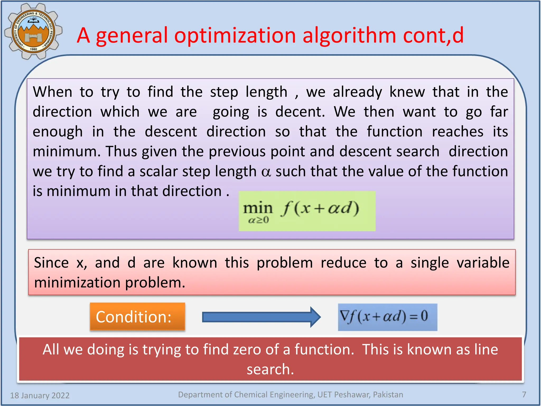
When to try to find the step length , we already knew that in the
direction which we are going is decent. We then want to go far
enough in the descent direction so that the function reaches its
minimum. Thus given the previous point and descent search direction
we try to find a scalar step length α such that the value of the function
is minimum in that direction .
18 January 2022 Department of Chemical Engineering, UET Peshawar, Pakistan 7
Since x, and d are known this problem reduce to a single variable
minimization problem.
Condition:
All we doing is trying to find zero of a function. This is known as line
search.
8.
Numerical precision
• Solvingthe first order optimality condition f(x*) = 0 is
equivalent to find the roots of the first derivative of the
function to be minimized.
18 January 2022 Department of Chemical Engineering, UET Peshawar, Pakistan 8
When we use computers it may not always be possible to
find the exact zero due to restriction on mechanic precision .
So we will be satisfied with finding x* that belongs to an
interval [ a, b ] such that the function f satisfies .
9.
Scaling
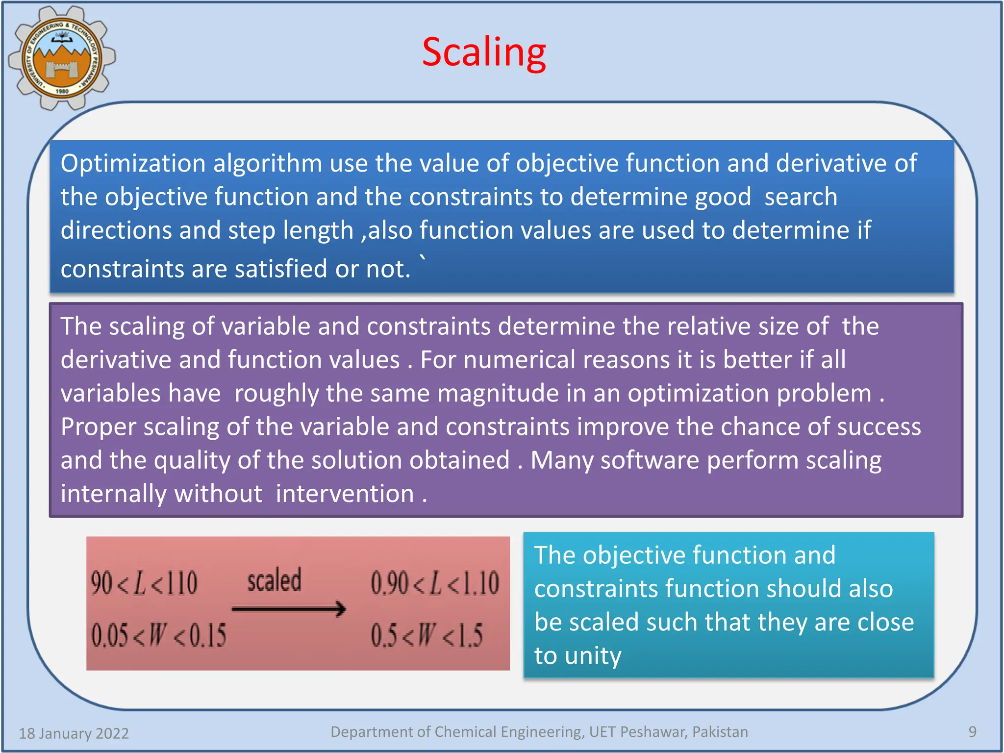
Optimization algorithm usethe value of objective function and derivative of
the objective function and the constraints to determine good search
directions and step length ,also function values are used to determine if
constraints are satisfied or not. `
18 January 2022 Department of Chemical Engineering, UET Peshawar, Pakistan 9
The scaling of variable and constraints determine the relative size of the
derivative and function values . For numerical reasons it is better if all
variables have roughly the same magnitude in an optimization problem .
Proper scaling of the variable and constraints improve the chance of success
and the quality of the solution obtained . Many software perform scaling
internally without intervention .
The objective function and
constraints function should also
be scaled such that they are close
to unity
10.
Convergence Rate
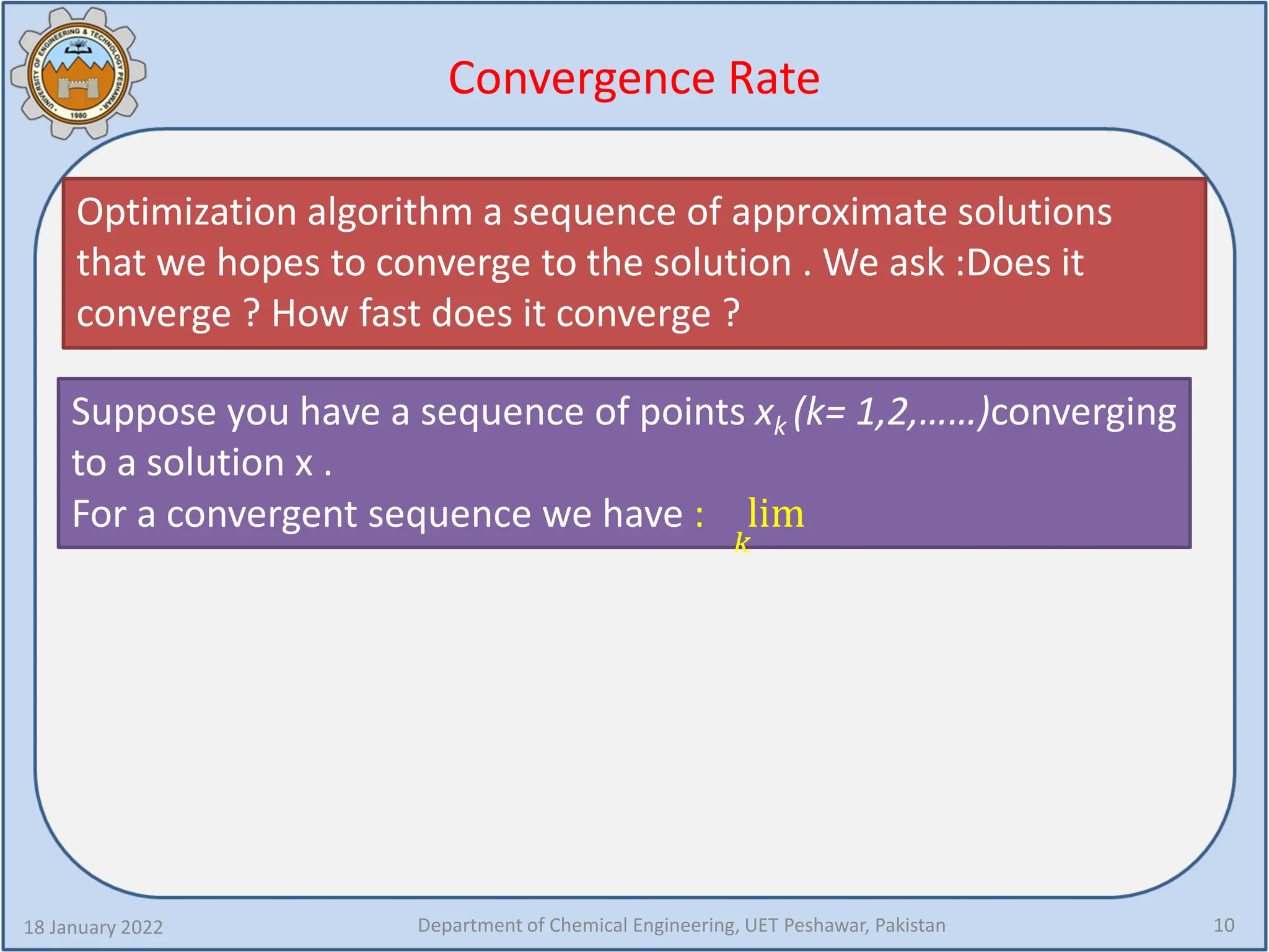
Optimization algorithma sequence of approximate solutions
that we hopes to converge to the solution . We ask :Does it
converge ? How fast does it converge ?
18 January 2022 Department of Chemical Engineering, UET Peshawar, Pakistan 10
Suppose you have a sequence of points xk (k= 1,2,……)converging
to a solution x .
For a convergent sequence we have : lim
𝑘𝑘
11.
Convergence Rate: cont,d
18January 2022
11
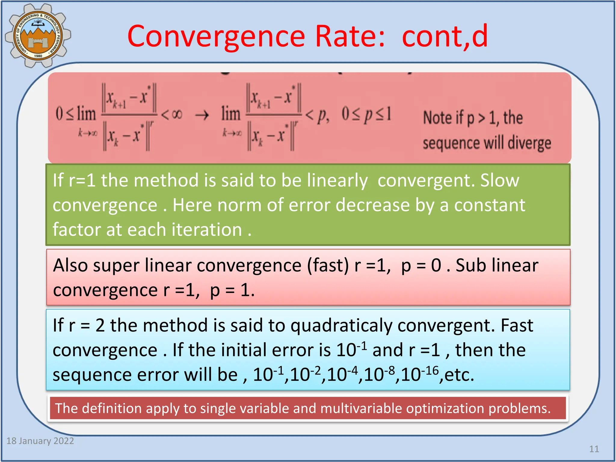
If r=1 the method is said to be linearly convergent. Slow
convergence . Here norm of error decrease by a constant
factor at each iteration .
Also super linear convergence (fast) r =1, p = 0 . Sub linear
convergence r =1, p = 1.
If r = 2 the method is said to quadraticaly convergent. Fast
convergence . If the initial error is 10-1 and r =1 , then the
sequence error will be , 10-1,10-2,10-4,10-8,10-16,etc.
The definition apply to single variable and multivariable optimization problems.
12.
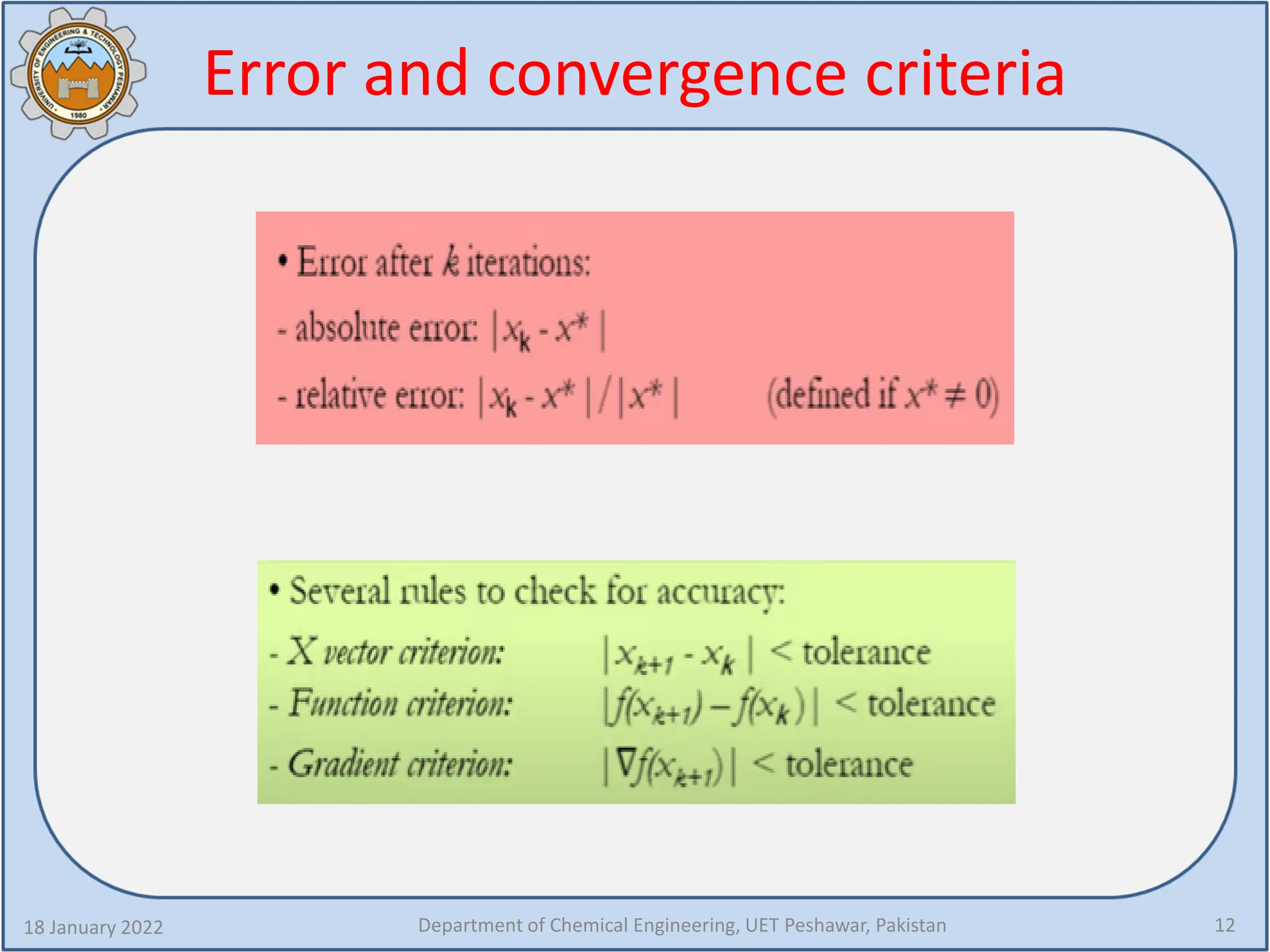
Error and convergencecriteria
18 January 2022 Department of Chemical Engineering, UET Peshawar, Pakistan 12
13.
Unconstrained single variableoptimization
method : A general classification
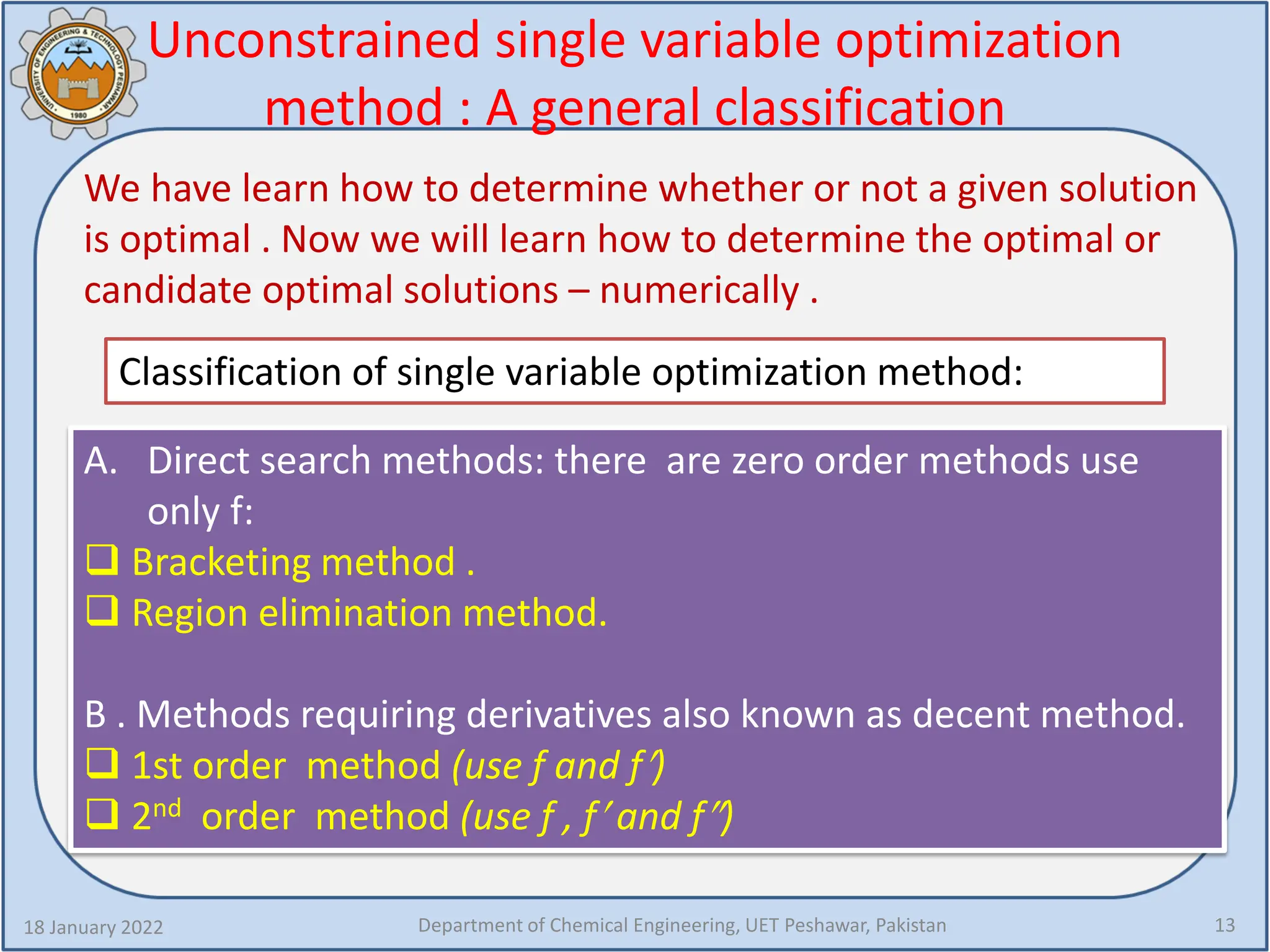
We have learn how to determine whether or not a given solution
is optimal . Now we will learn how to determine the optimal or
candidate optimal solutions – numerically .
18 January 2022 Department of Chemical Engineering, UET Peshawar, Pakistan 13
Classification of single variable optimization method:
A. Direct search methods: there are zero order methods use
only f:
Bracketing method .
Region elimination method.
B . Methods requiring derivatives also known as decent method.
1st order method (use f and f′)
2nd order method (use f , f′ and f″)
14.
Unimodality and bracketingthe optimum
18 January 2022 Department of Chemical Engineering, UET Peshawar, Pakistan 14
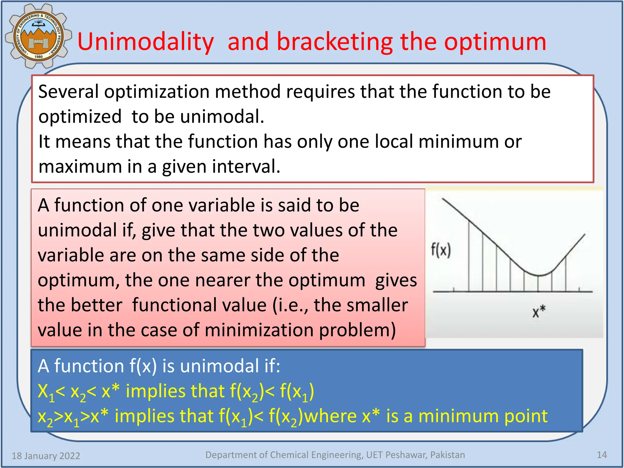
Several optimization method requires that the function to be
optimized to be unimodal.
It means that the function has only one local minimum or
maximum in a given interval.
A function of one variable is said to be
unimodal if, give that the two values of the
variable are on the same side of the
optimum, the one nearer the optimum gives
the better functional value (i.e., the smaller
value in the case of minimization problem)
A function f(x) is unimodal if:
X1< x2< x* implies that f(x2)< f(x1)
x2>x1>x* implies that f(x1)< f(x2)where x* is a minimum point
15.
Bracketing method :exhaustive search
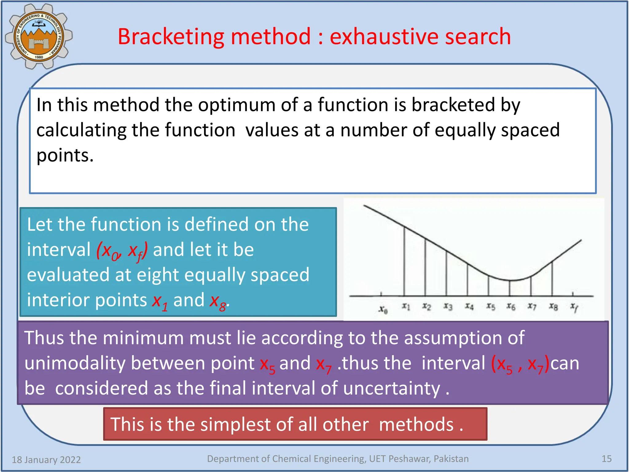
In this method the optimum of a function is bracketed by
calculating the function values at a number of equally spaced
points.
18 January 2022 Department of Chemical Engineering, UET Peshawar, Pakistan 15
Let the function is defined on the
interval (x0, xf) and let it be
evaluated at eight equally spaced
interior points x1 and x8.
Thus the minimum must lie according to the assumption of
unimodality between point x5 and x7 .thus the interval (x5 , x7)can
be considered as the final interval of uncertainty .
This is the simplest of all other methods .
16.
Exhaustive search method:Algorithm
18 January 2022 Department of Chemical Engineering, UET Peshawar, Pakistan 16
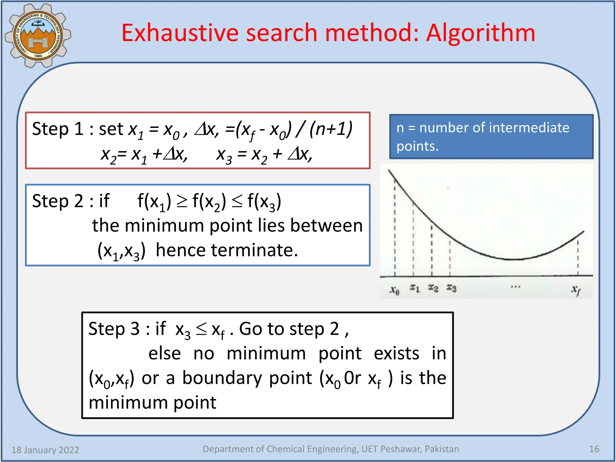
Step 1 : set x1 = x0 , ∆x, =(xf - x0) / (n+1)
x2= x1 +∆x, x3 = x2 + ∆x,
Step 2 : if f(x1) ≥ f(x2) ≤ f(x3)
the minimum point lies between
(x1,x3) hence terminate.
Step 3 : if x3 ≤ xf . Go to step 2 ,
else no minimum point exists in
(x0,xf) or a boundary point (x0 0r xf ) is the
minimum point
n = number of intermediate
points.
17.
Exhaustive search method:Algorithm
18 January 2022 Department of Chemical Engineering, UET Peshawar, Pakistan 17
In the interval (x0 ,xf) the objective function has been
evaluated at n equally spaced point:
X0< X1 <X2 … <Xn <Xf
If the minimum value among the n
function values is xk then the final
interval of uncertainty is [xk-1, xk+1]
with length of :
18.
Exhaustive search method:example 1
18 January 2022 Department of Chemical Engineering, UET Peshawar, Pakistan 18
Find the minimum of 𝑓𝑓 𝑥𝑥 = 𝑥𝑥 𝑥𝑥 − 1.5
in the interval [0,1] to within 10 % of the
exact value .
Plot x vs f(x) for
x=0 to x=1
19.
Exhaustive search method:example 1 cont,d
18 January 2022 Department of Chemical Engineering, UET Peshawar, Pakistan 19
Find the minimum of 𝑓𝑓 𝑥𝑥 = 𝑥𝑥 𝑥𝑥 − 1.5 in the interval
[1,2] to within 10 % of the exact value.
Solution:
If the middle point of the final interval of uncertainty is taken as
the approximate point , the maximum deviation could 1/n+1
times the interval of uncertainty . Thus to find the optimum with
in 10% of the exact value we should have :
20.
Exhaustive search method:homework
18 January 2022 Department of Chemical Engineering, UET Peshawar, Pakistan 20
21.
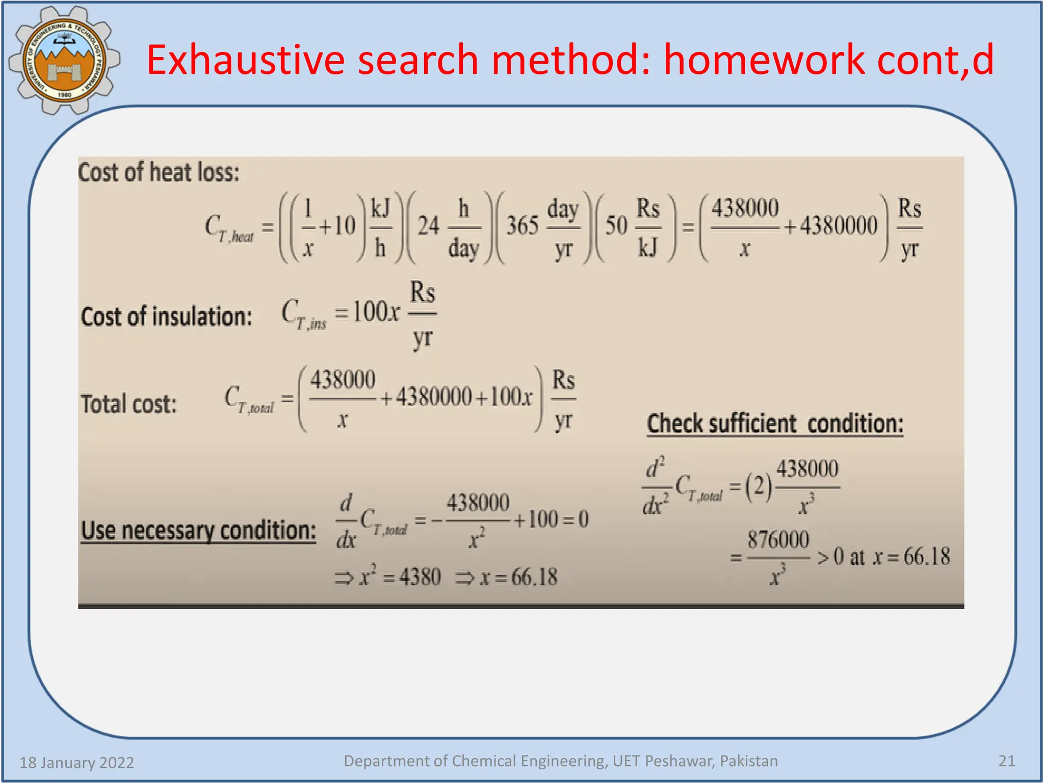
Exhaustive search method:homework cont,d
18 January 2022 Department of Chemical Engineering, UET Peshawar, Pakistan 21
22.
Scanning and bracketingthe optimum
18 January 2022 Department of Chemical Engineering, UET Peshawar, Pakistan 22
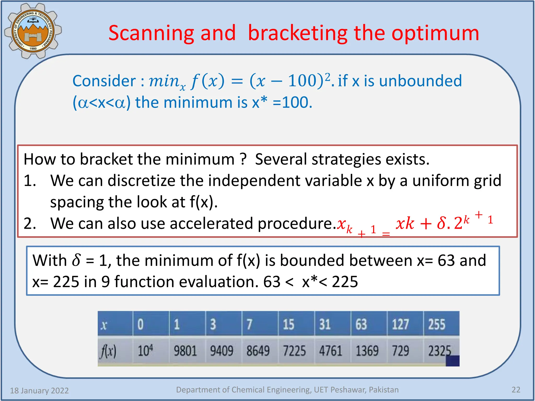
Consider : 𝑚𝑚𝑚𝑚𝑚𝑚𝑥𝑥 𝑓𝑓 𝑥𝑥 = 𝑥𝑥 − 100 2. if x is unbounded
(α<x<α) the minimum is x* =100.
How to bracket the minimum ? Several strategies exists.
1. We can discretize the independent variable x by a uniform grid
spacing the look at f(x).
2. We can also use accelerated procedure.𝑥𝑥𝑘𝑘 + 1 =
𝑥𝑥𝑥𝑥 + 𝛿𝛿. 2𝑘𝑘 + 1
With 𝛿𝛿 = 1, the minimum of f(x) is bounded between x= 63 and
x= 225 in 9 function evaluation. 63 < x*< 225
23.
Bracketing method :Bounding phase method
18 January 2022 Department of Chemical Engineering, UET Peshawar, Pakistan 23
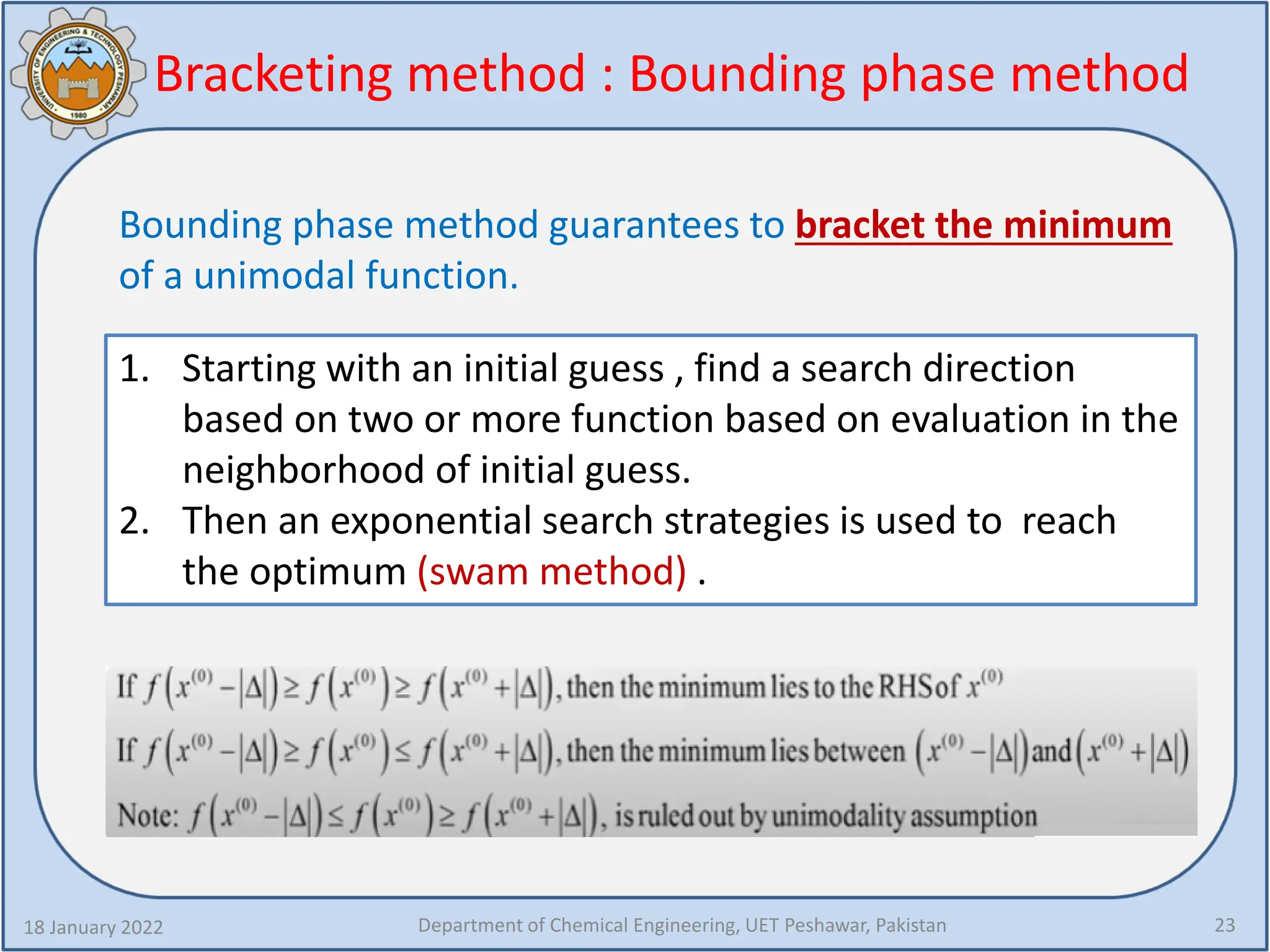
Bounding phase method guarantees to bracket the minimum
of a unimodal function.
1. Starting with an initial guess , find a search direction
based on two or more function based on evaluation in the
neighborhood of initial guess.
2. Then an exponential search strategies is used to reach
the optimum (swam method) .
24.
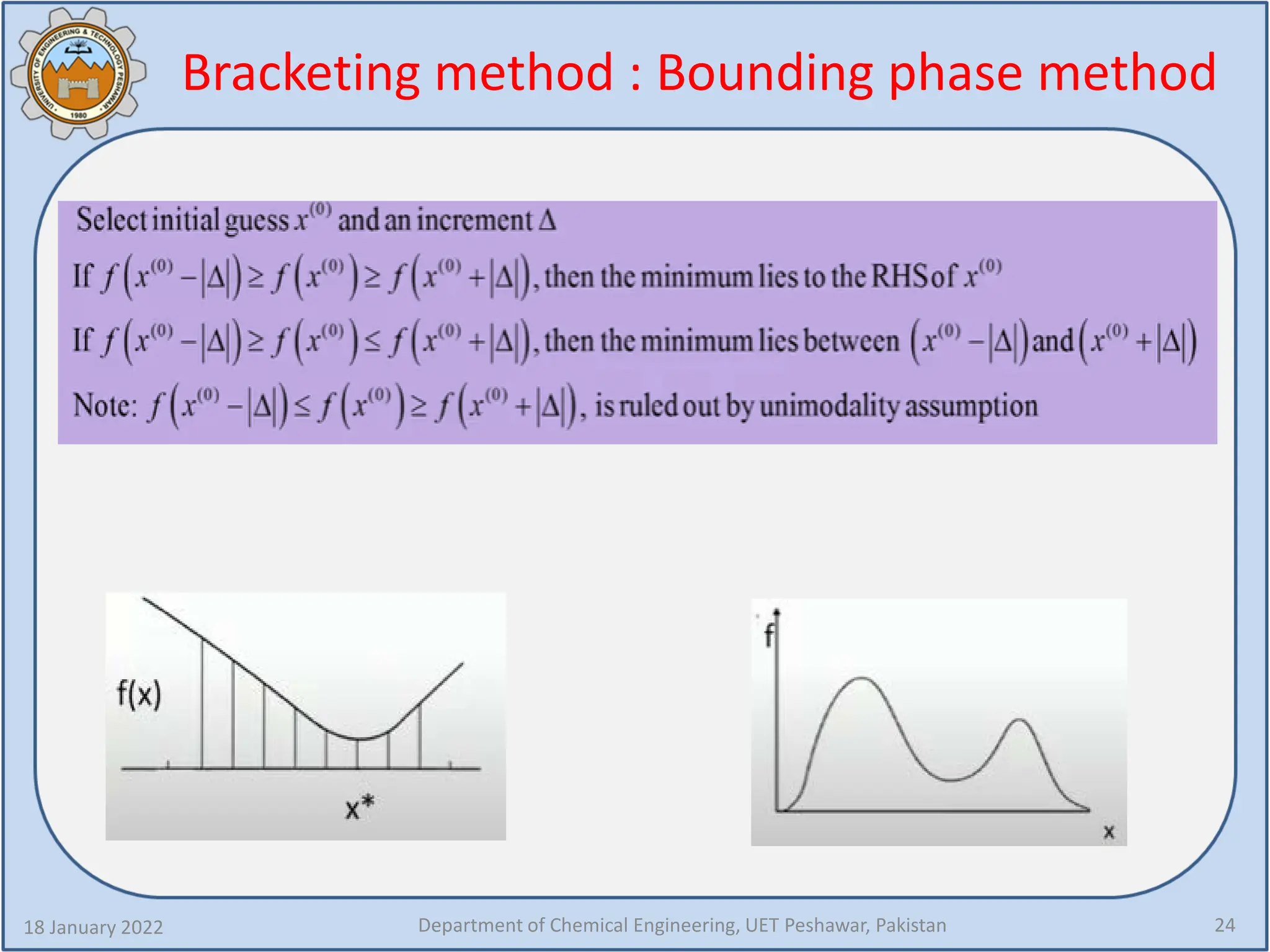
Bracketing method :Bounding phase method
18 January 2022 Department of Chemical Engineering, UET Peshawar, Pakistan 24
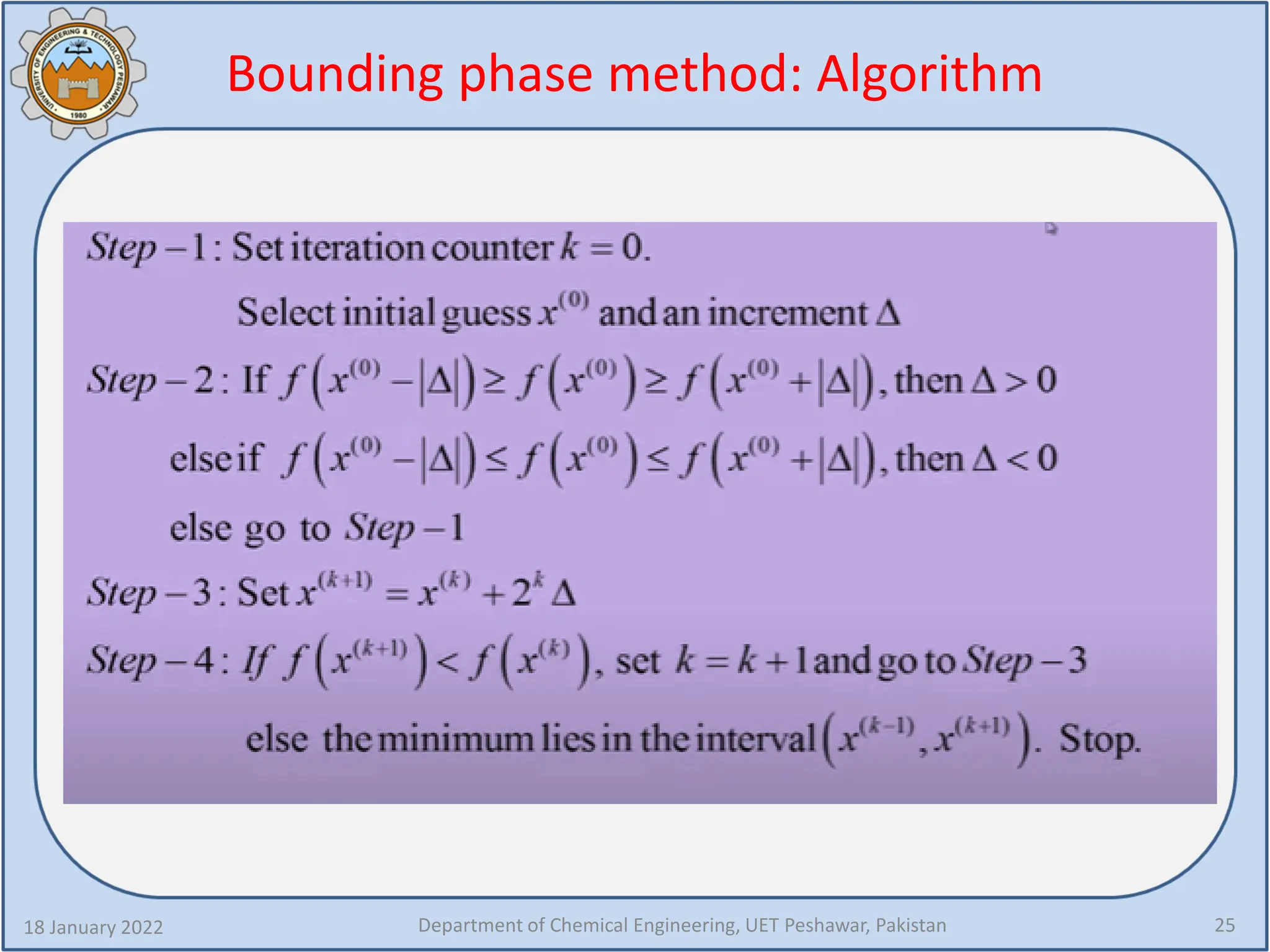
25.
Bounding phase method:Algorithm
18 January 2022 Department of Chemical Engineering, UET Peshawar, Pakistan 25
26.
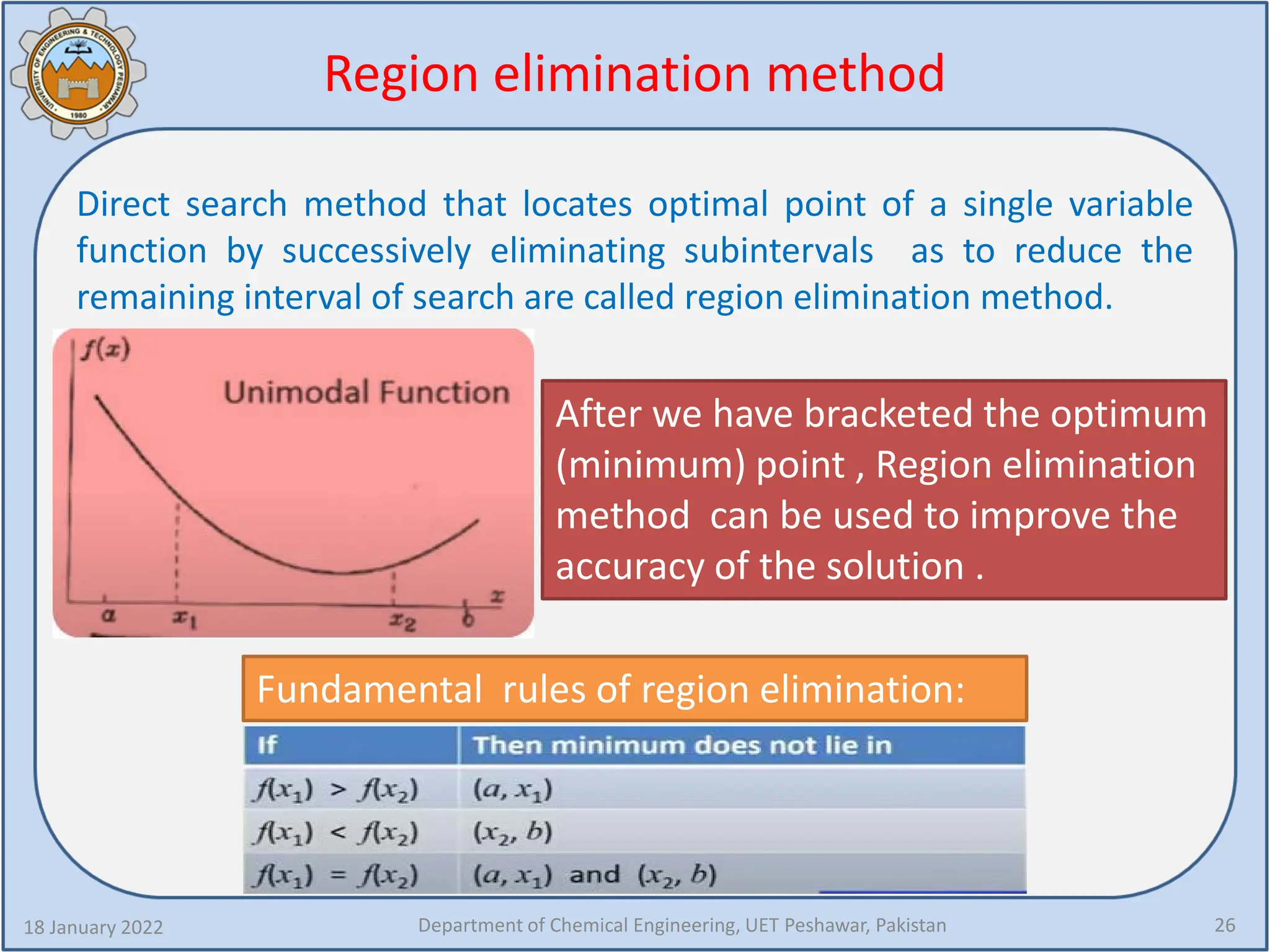
Region elimination method
18January 2022 Department of Chemical Engineering, UET Peshawar, Pakistan 26
After we have bracketed the optimum
(minimum) point , Region elimination
method can be used to improve the
accuracy of the solution .
Direct search method that locates optimal point of a single variable
function by successively eliminating subintervals as to reduce the
remaining interval of search are called region elimination method.
Fundamental rules of region elimination:
27.
Region elimination method: How to place trial
points
18 January 2022 Department of Chemical Engineering, UET Peshawar, Pakistan 27
Fundamental rules of region elimination:
Note that depending on function value we will delete [a, x1]
,[x2,b] or both. In order to reduce interval of uncertainty ,we
would like to maximize the length of [a, x1] or ,[x2,b] .To maximize
both we should place x1 and x2 symmetrically in the interval
[a,b].
28.
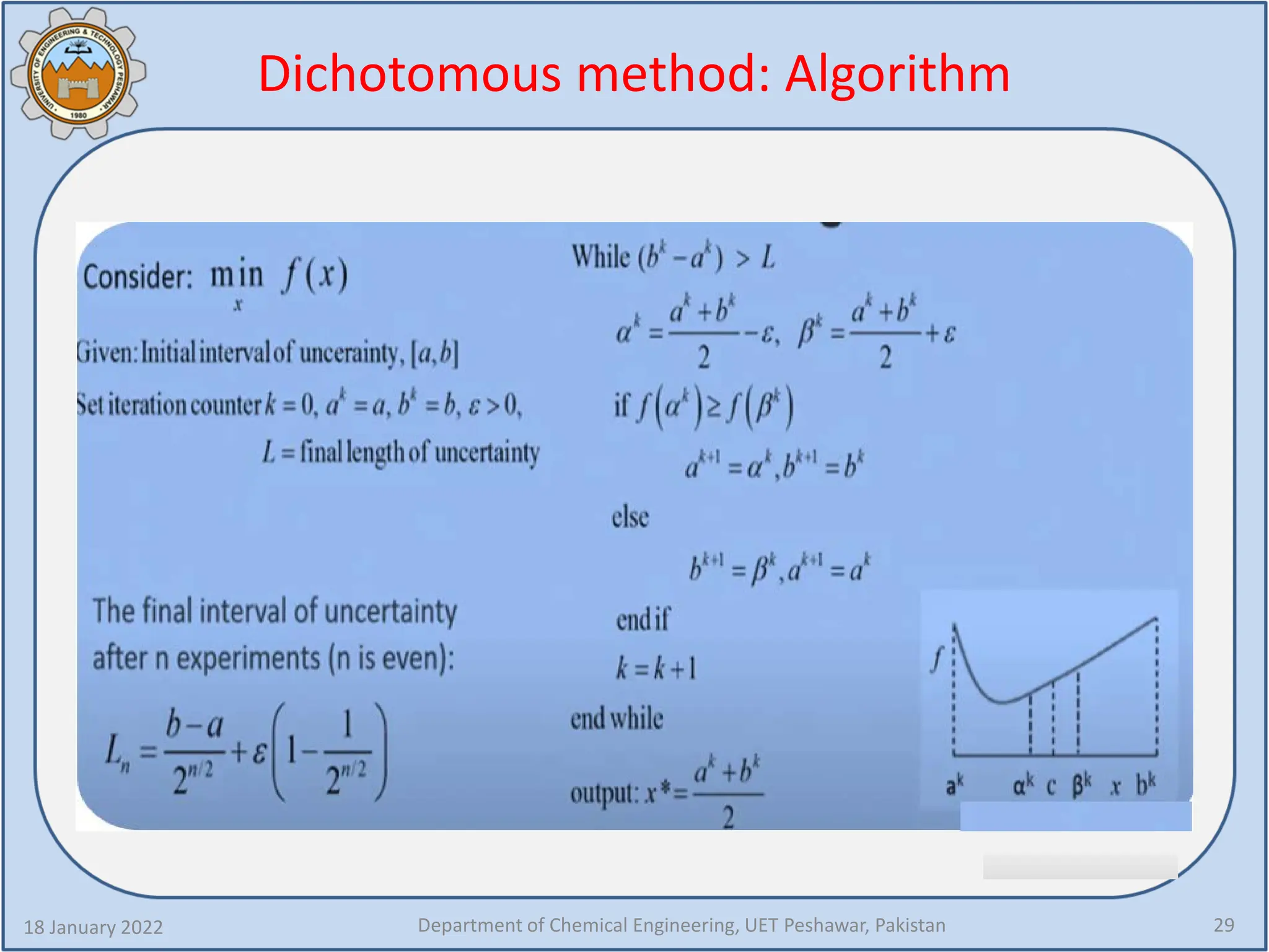
Region elimination method: Dichotomous search
18 January 2022 Department of Chemical Engineering, UET Peshawar, Pakistan 28
Let the optimum lie between [a,b]. The dichotomous
method first compute the mid point a+b//2 and then move
slightly to either side of the mid-point to compute two test
points : a+b/2 +
� ε.
Based on the function values and
unimodality assumptions, the
interval is updated by eliminating
one part and the procedure
continuous until the optimal
solution is contained in a small
interval.
This method is also known as method of bisecting.
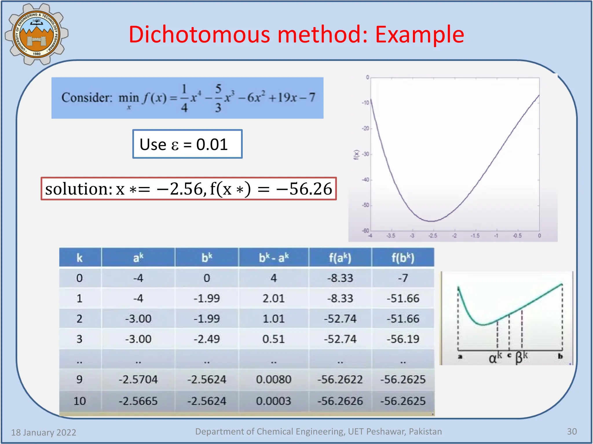
Dichotomous method: Example
18January 2022 Department of Chemical Engineering, UET Peshawar, Pakistan 30
solution: x ∗= −2.56, f x ∗ = −56.26
Use ε = 0.01
31.
Region elimination: intervalhalving method
18 January 2022 Department of Chemical Engineering, UET Peshawar, Pakistan 31
Once the optimum has been bracketed, region elimination
method give us a more refined estimate of the optimum by
eliminating certain amount of subinterval at each step.
Internal halving method
eliminate exactly one-half of
the interval at each stage
by considering three equally
spaced trail points. These
three points divide the
interval [a,b] into 4 equal
regions.
32.
18 January 2022Department of Chemical Engineering, UET Peshawar, Pakistan 32
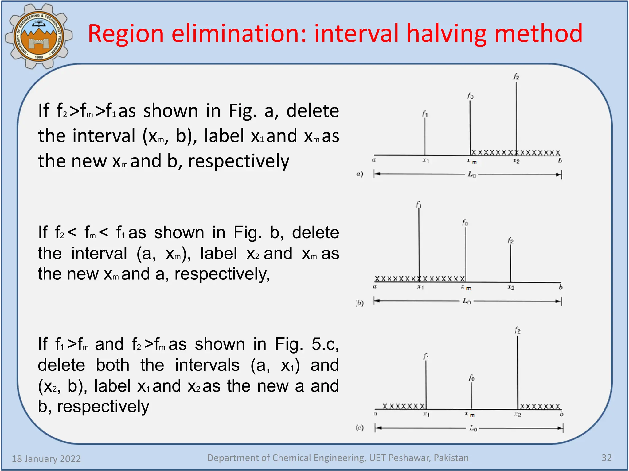
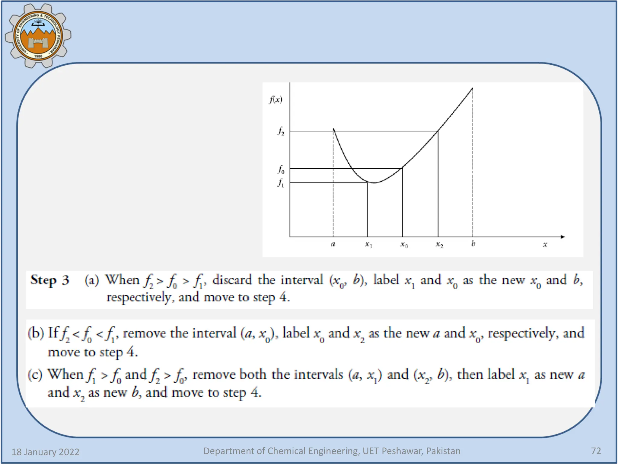
If f2 >fm >f1 as shown in Fig. a, delete
the interval (xm, b), label x1 and xm as
the new xm and b, respectively
If f2 < fm < f1 as shown in Fig. b, delete
the interval (a, xm), label x2 and xm as
the new xm and a, respectively,
If f1 >fm and f2 >fm as shown in Fig. 5.c,
delete both the intervals (a, x1) and
(x2, b), label x1 and x2 as the new a and
b, respectively
Region elimination: interval halving method
33.
Region elimination intervalhalving method:
Algorithm
18 January 2022 Department of Chemical Engineering, UET Peshawar, Pakistan 33
Step-3: If f(x1) < f(xm), set xm = b; and x1 = xm; go to step-5;
Else go step-2, step, 4
Step-4: If f(x2) < f(xm), set xm = a; and x2 = xm; go to step-5;
Else set x1 = a; x2 = b; go to step-5
Step-5: Evaluate L = (b - a), if I L I < ɛ, stop;
Else go to step-2
Step-2: Set x1 = a + L/4, x2 = b – L/4. Evaluate f(x1), f(x2)
Step-1: Given x* Є [a, b], L0 = L = (b-a), ɛ > 0
Let xm = (a + b)/2; Evaluate f(xm)
34.
Interval halving methodAnalysis
18 January 2022 Department of Chemical Engineering, UET Peshawar, Pakistan 34
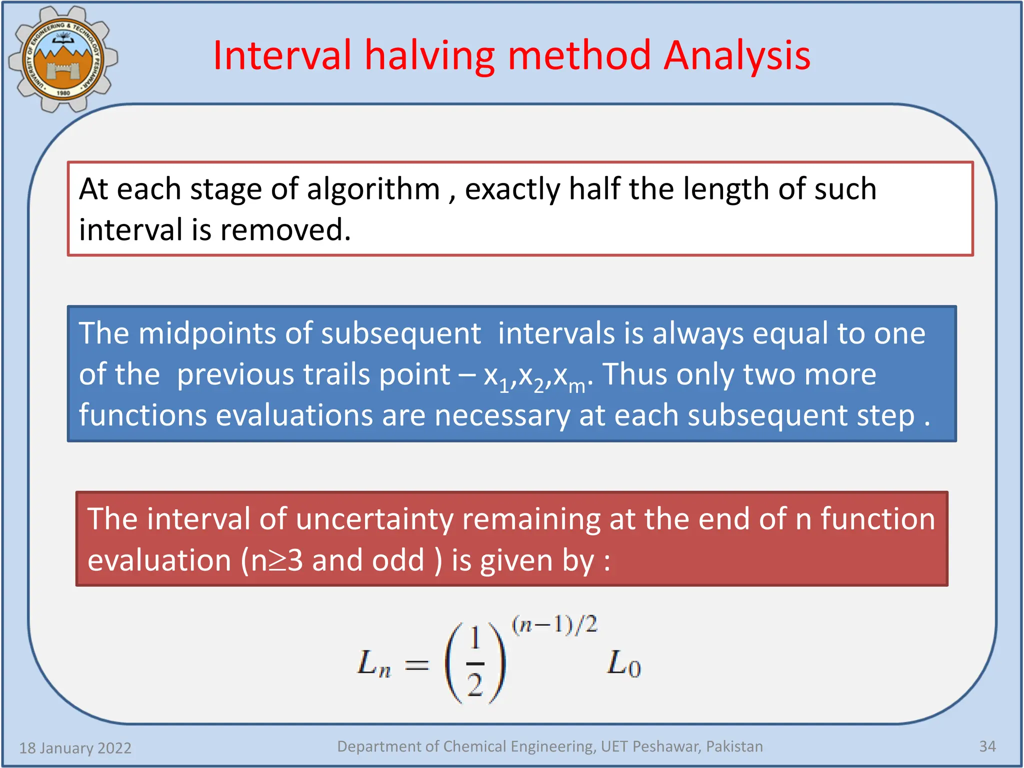
At each stage of algorithm , exactly half the length of such
interval is removed.
The midpoints of subsequent intervals is always equal to one
of the previous trails point – x1,x2,xm. Thus only two more
functions evaluations are necessary at each subsequent step .
The interval of uncertainty remaining at the end of n function
evaluation (n≥3 and odd ) is given by :
35.
Interval halving methodexample
Find the minimum of 𝑓𝑓 𝑥𝑥 = 𝑥𝑥 𝑥𝑥 − 1.5 in the interval [0,1] to
within 10 % of the exact value.
Solution:
If the middle point of the final interval of uncertainty is taken as
the optimum point , the specified accuracy can be achieved if
18 January 2022 Department of Chemical Engineering, UET Peshawar, Pakistan 35
and also,
36.
18 January 2022Department of Chemical Engineering, UET Peshawar, Pakistan 36
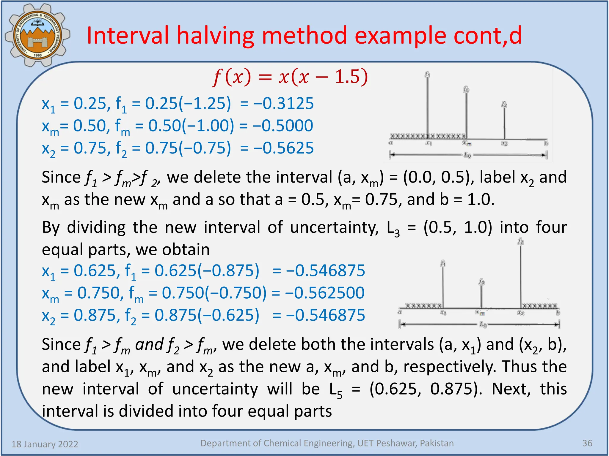
x1 = 0.25, f1 = 0.25(−1.25) = −0.3125
xm= 0.50, fm = 0.50(−1.00) = −0.5000
x2 = 0.75, f2 = 0.75(−0.75) = −0.5625
Since f1 > fm>f 2, we delete the interval (a, xm) = (0.0, 0.5), label x2 and
xm as the new xm and a so that a = 0.5, xm= 0.75, and b = 1.0.
x1 = 0.625, f1 = 0.625(−0.875) = −0.546875
xm = 0.750, fm = 0.750(−0.750) = −0.562500
x2 = 0.875, f2 = 0.875(−0.625) = −0.546875
Since f1 > fm and f2 > fm, we delete both the intervals (a, x1) and (x2, b),
and label x1, xm, and x2 as the new a, xm, and b, respectively. Thus the
new interval of uncertainty will be L5 = (0.625, 0.875). Next, this
interval is divided into four equal parts
Interval halving method example cont,d
𝑓𝑓 𝑥𝑥 = 𝑥𝑥 𝑥𝑥 − 1.5
By dividing the new interval of uncertainty, L3 = (0.5, 1.0) into four
equal parts, we obtain
37.
18 January 2022Department of Chemical Engineering, UET Peshawar, Pakistan 37
Interval halving method example cont,d
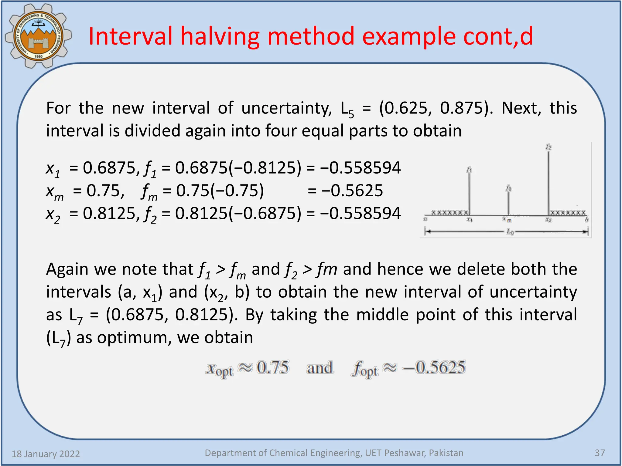
For the new interval of uncertainty, L5 = (0.625, 0.875). Next, this
interval is divided again into four equal parts to obtain
x1 = 0.6875, f1 = 0.6875(−0.8125) = −0.558594
xm = 0.75, fm = 0.75(−0.75) = −0.5625
x2 = 0.8125, f2 = 0.8125(−0.6875) = −0.558594
Again we note that f1 > fm and f2 > fm and hence we delete both the
intervals (a, x1) and (x2, b) to obtain the new interval of uncertainty
as L7 = (0.6875, 0.8125). By taking the middle point of this interval
(L7) as optimum, we obtain
38.
Interval halving methodHomework
Consider 𝑓𝑓 𝑥𝑥 = 100 − 𝑥𝑥2 .
Find xopt by interval halving method. Take x=[60,150].
Note xopt = 100.
Perform 3 iteration and see that the mid point of the interval
after 3 iterations is already 99.375.
18 January 2022 Department of Chemical Engineering, UET Peshawar, Pakistan 38
39.
18 January 2022Department of Chemical Engineering, UET Peshawar, Pakistan 39
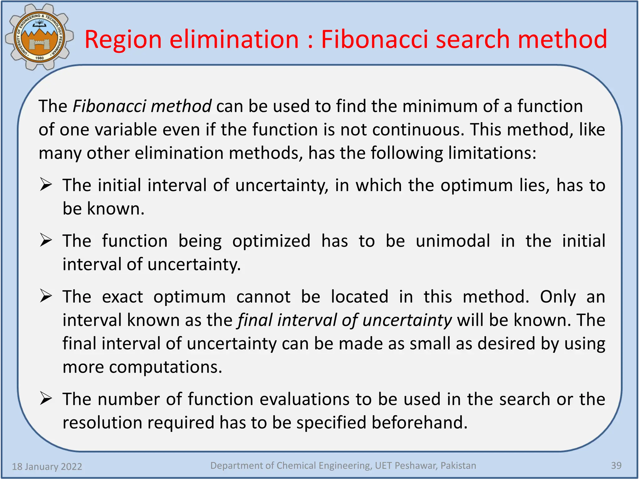
The Fibonacci method can be used to find the minimum of a function
of one variable even if the function is not continuous. This method, like
many other elimination methods, has the following limitations:
The initial interval of uncertainty, in which the optimum lies, has to
be known.
The function being optimized has to be unimodal in the initial
interval of uncertainty.
The exact optimum cannot be located in this method. Only an
interval known as the final interval of uncertainty will be known. The
final interval of uncertainty can be made as small as desired by using
more computations.
The number of function evaluations to be used in the search or the
resolution required has to be specified beforehand.
Region elimination : Fibonacci search method
40.
Region elimination :Fibonacci search method
18 January 2022 Department of Chemical Engineering, UET Peshawar, Pakistan 40
Fibonacci search methods use the sequence of
Fibonacci numbers [Fn], to reduce the interval of
uncertainty. These numbers are defined as:
𝐹𝐹0 = 𝐹𝐹1 = 1
𝐹𝐹𝑛𝑛 = 𝐹𝐹 𝑛𝑛 − 1 +
𝐹𝐹𝑛𝑛 − 2,
𝑛𝑛 = 2, 3, 4 …
Each number after the first two represent the sum of the
proceeding two.
First few Fibonacci numbers are 1, 1, 2, 3, 5, 8, 13, 21, 34, 55, 89,…
41.
Fibonacci search method: How does it work?
18 January 2022 Department of Chemical Engineering, UET Peshawar, Pakistan 41
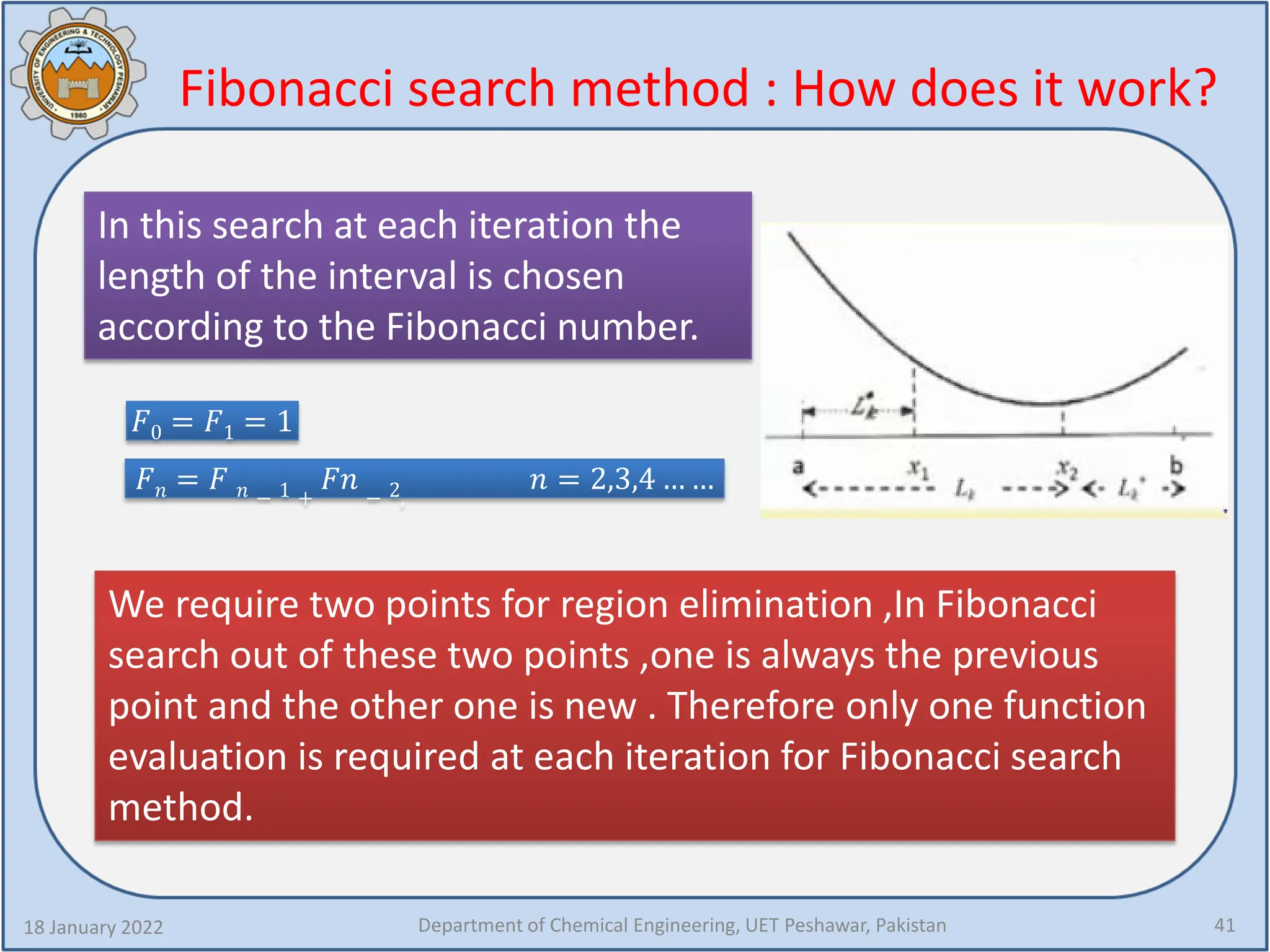
In this search at each iteration the
length of the interval is chosen
according to the Fibonacci number.
𝐹𝐹0 = 𝐹𝐹1 = 1
𝐹𝐹𝑛𝑛 = 𝐹𝐹 𝑛𝑛 − 1 +
𝐹𝐹𝐹𝐹 − 2,
𝑛𝑛 = 2,3,4 … …
We require two points for region elimination ,In Fibonacci
search out of these two points ,one is always the previous
point and the other one is new . Therefore only one function
evaluation is required at each iteration for Fibonacci search
method.
42.
Fibonacci search methodhow does it work?
18 January 2022 Department of Chemical Engineering, UET Peshawar, Pakistan 42
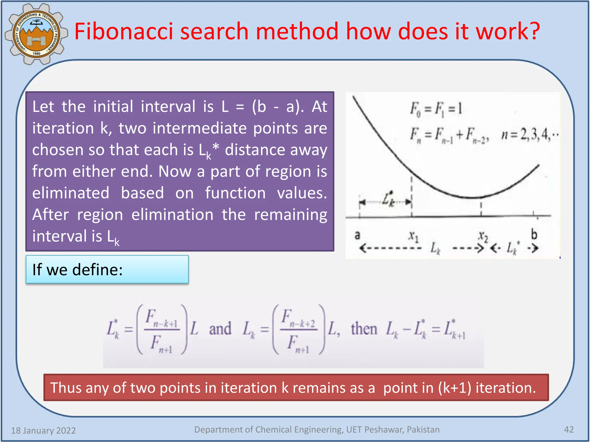
Let the initial interval is L = (b - a). At
iteration k, two intermediate points are
chosen so that each is Lk* distance away
from either end. Now a part of region is
eliminated based on function values.
After region elimination the remaining
interval is Lk
If we define:
Thus any of two points in iteration k remains as a point in (k+1) iteration.
43.
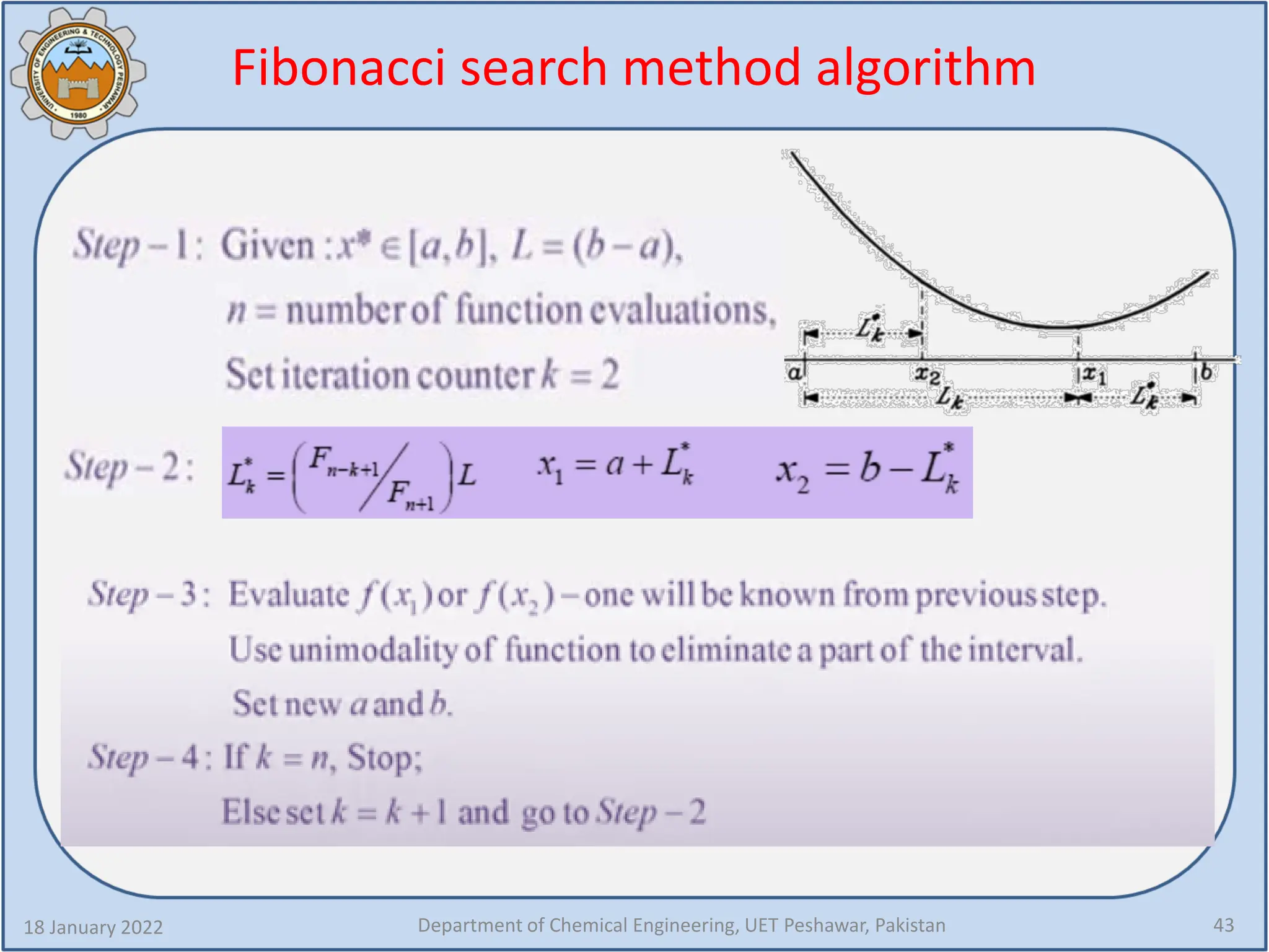
Fibonacci search methodalgorithm
18 January 2022 Department of Chemical Engineering, UET Peshawar, Pakistan 43
44.
Fibonacci search method: Analysis
18 January 2022 Department of Chemical Engineering, UET Peshawar, Pakistan 44
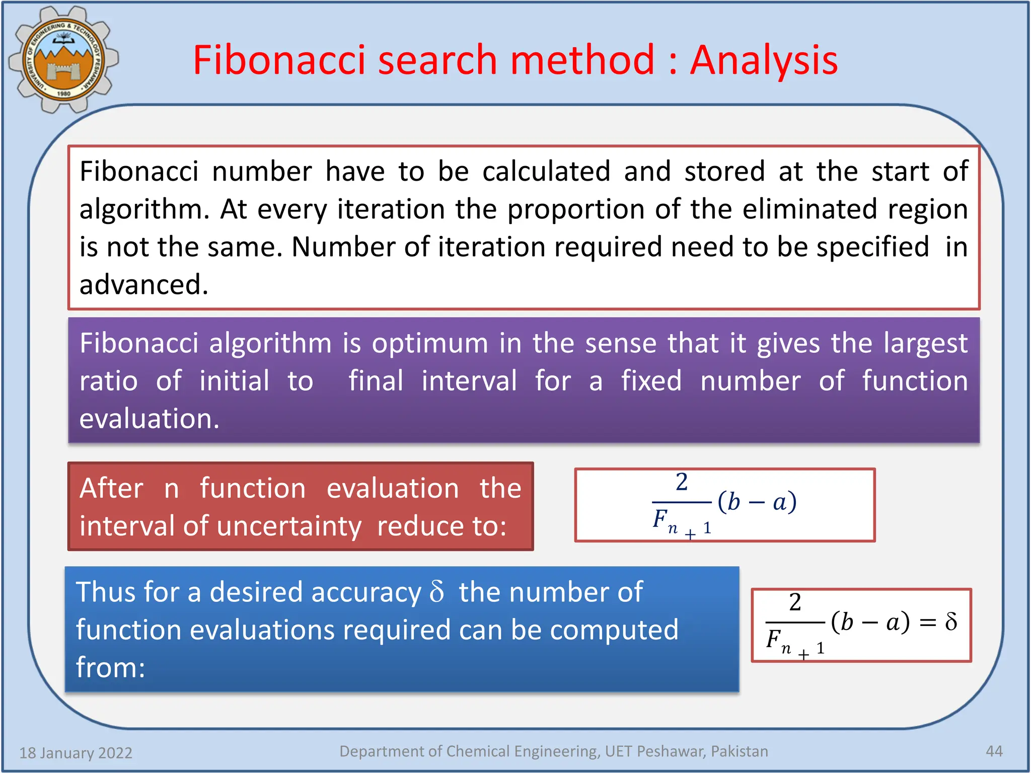
Fibonacci number have to be calculated and stored at the start of
algorithm. At every iteration the proportion of the eliminated region
is not the same. Number of iteration required need to be specified in
advanced.
Fibonacci algorithm is optimum in the sense that it gives the largest
ratio of initial to final interval for a fixed number of function
evaluation.
After n function evaluation the
interval of uncertainty reduce to:
Thus for a desired accuracy δ the number of
function evaluations required can be computed
from:
2
𝐹𝐹𝑛𝑛 + 1
𝑏𝑏 − 𝑎𝑎
2
𝐹𝐹𝑛𝑛 + 1
𝑏𝑏 − 𝑎𝑎 = δ
45.
Fibonacci search method:example
18 January 2022 Department of Chemical Engineering, UET Peshawar, Pakistan 45
Using Fibonacci search method, minimize the following
function in the interval x = [1, 6]. Perform 3 iteration (n=3).
𝑚𝑚𝑚𝑚𝑚𝑚𝑥𝑥 𝑓𝑓 𝑥𝑥 = 𝑥𝑥2 +
30
𝑥𝑥
46.
Example cont,d
18 January2022 Department of Chemical Engineering, UET Peshawar, Pakistan 46
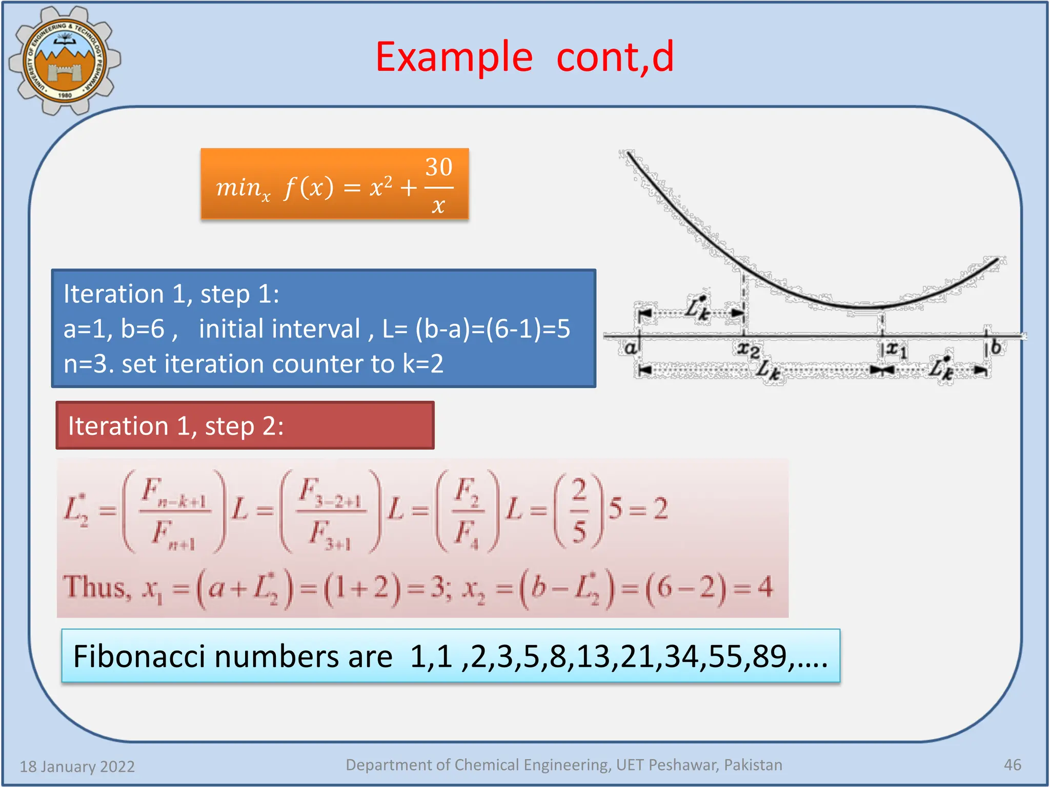
𝑚𝑚𝑚𝑚𝑚𝑚𝑥𝑥 𝑓𝑓 𝑥𝑥 = 𝑥𝑥2 +
30
𝑥𝑥
Iteration 1, step 1:
a=1, b=6 , initial interval , L= (b-a)=(6-1)=5
n=3. set iteration counter to k=2
Iteration 1, step 2:
Fibonacci numbers are 1,1 ,2,3,5,8,13,21,34,55,89,….
47.
Example cont,d
18 January2022 Department of Chemical Engineering, UET Peshawar, Pakistan 47
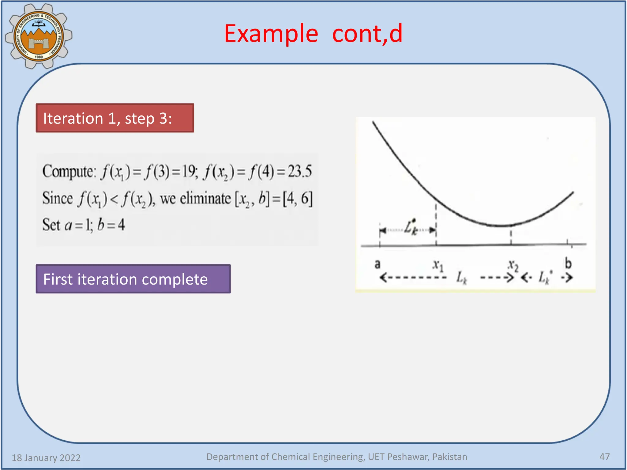
Iteration 1, step 3:
First iteration complete
48.
Example cont,d
18 January2022 Department of Chemical Engineering, UET Peshawar, Pakistan 48
Iteration 2, step 1:
Second iteration complete
Iteration 2, step 3:
Minimum is bracketed between [2,3] . In
actual practice we should consider higher
value of n and proceed as shown.
49.
Region elimination: Goldensection search
method
18 January 2022 Department of Chemical Engineering, UET Peshawar, Pakistan 49
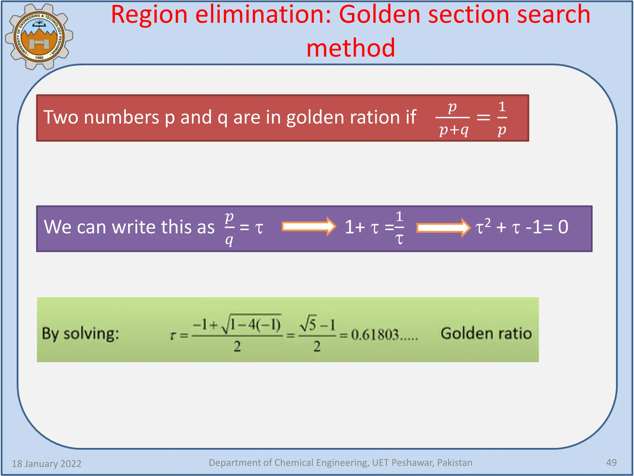
Two numbers p and q are in golden ration if
𝑝𝑝
𝑝𝑝+𝑞𝑞
=
1
𝑝𝑝
We can write this as
𝑝𝑝
𝑞𝑞
= τ 1+ τ =
1
τ
τ2 + τ -1= 0
50.
Golden section searchmethod: Golden ratio
18 January 2022 Department of Chemical Engineering, UET Peshawar, Pakistan 50
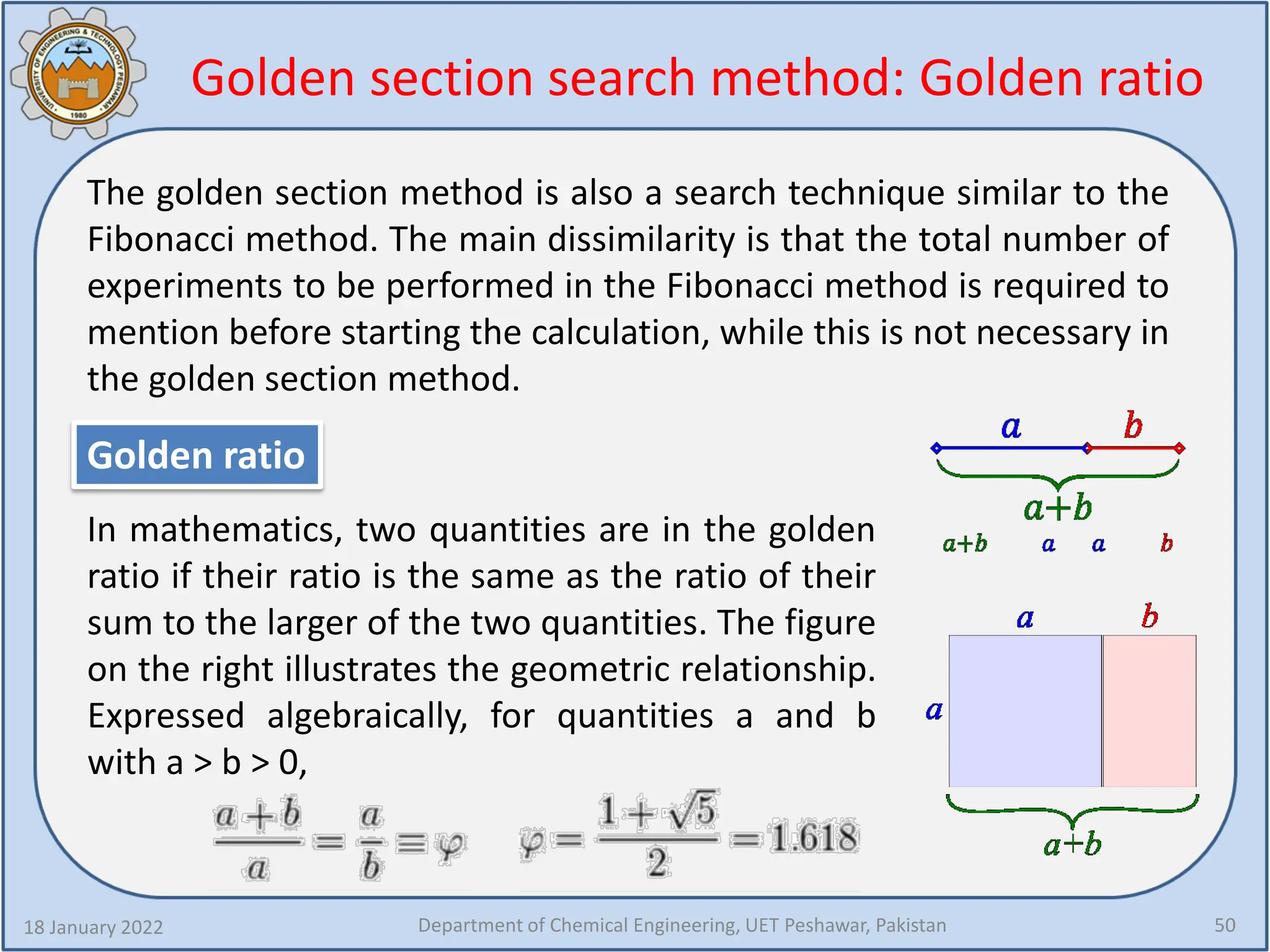
The golden section method is also a search technique similar to the
Fibonacci method. The main dissimilarity is that the total number of
experiments to be performed in the Fibonacci method is required to
mention before starting the calculation, while this is not necessary in
the golden section method.
Golden ratio
In mathematics, two quantities are in the golden
ratio if their ratio is the same as the ratio of their
sum to the larger of the two quantities. The figure
on the right illustrates the geometric relationship.
Expressed algebraically, for quantities a and b
with a > b > 0,
51.
Golden ratio andFibonacci number
18 January 2022 Department of Chemical Engineering, UET Peshawar, Pakistan 51
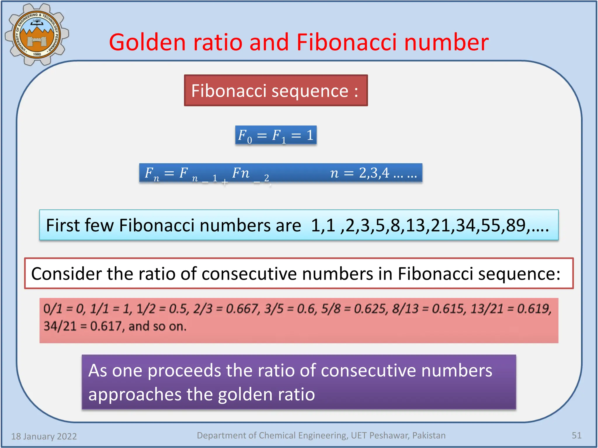
𝐹𝐹0 = 𝐹𝐹1 = 1
𝐹𝐹𝑛𝑛 = 𝐹𝐹 𝑛𝑛 − 1 +
𝐹𝐹𝐹𝐹 − 2,
𝑛𝑛 = 2,3,4 … …
First few Fibonacci numbers are 1,1 ,2,3,5,8,13,21,34,55,89,….
Fibonacci sequence :
Consider the ratio of consecutive numbers in Fibonacci sequence:
As one proceeds the ratio of consecutive numbers
approaches the golden ratio
52.
Golden section searchmethod : Algorithm
18 January 2022 Department of Chemical Engineering, UET Peshawar, Pakistan 52
τ 1 − τ
1. Start with a unit interval of convenience. Thus the given interval may be
scaled up to [0,1]. .
2. Place two trail points a friction τ from either end.
3. Suppose RHS interval is eliminated he remaining subinterval has length τ
and it has an old trial point located interior to it at a distance (1- τ ) from
the left end point.
4. Each subsequent iteration will eliminate (1- τ ) of the remaining interval
.thus after n function evaluation the interval remaining will be ( τn-1 )
53.
Golden section searchmethod algorithm
18 January 2022 Department of Chemical Engineering, UET Peshawar, Pakistan 53
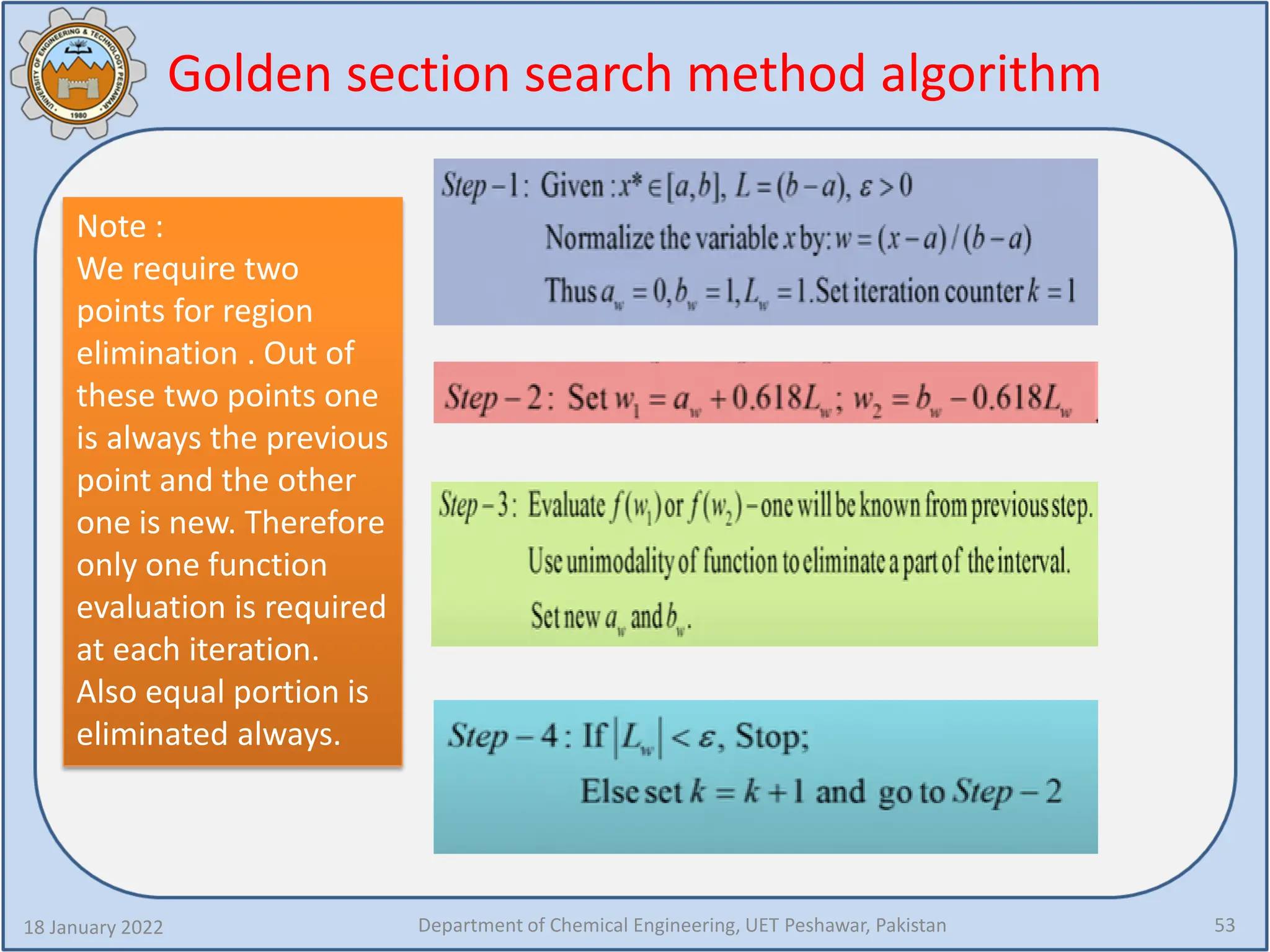
Note :
We require two
points for region
elimination . Out of
these two points one
is always the previous
point and the other
one is new. Therefore
only one function
evaluation is required
at each iteration.
Also equal portion is
eliminated always.
54.
Golden section searchmethod : Example
18 January 2022 Department of Chemical Engineering, UET Peshawar, Pakistan 54
minx f x = 100 − x 2 60 ≤ x ≤ 150
Solution:
Let us first scale the interval [60,150] to [0,1] and
reformulate the problem:
𝑤𝑤 =
𝑥𝑥−60
150−60
=
𝑥𝑥−60
90
minx f w = 40 − 90𝑤𝑤 2, 0 ≤ w ≤ 1
55.
Golden section searchmethod : Example
18 January 2022 Department of Chemical Engineering, UET Peshawar, Pakistan 55
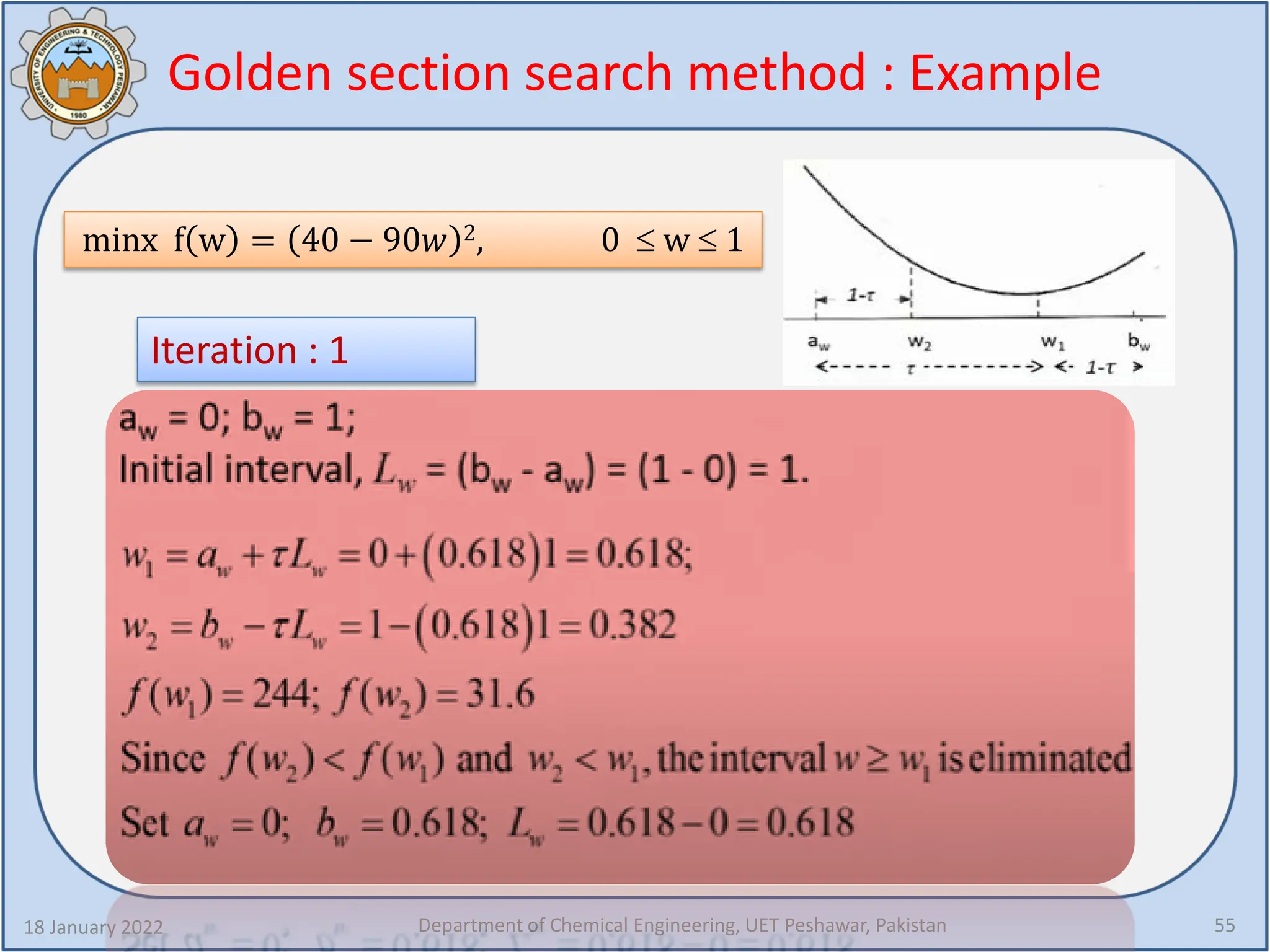
minx f w = 40 − 90𝑤𝑤 2, 0 ≤ w ≤ 1
Iteration : 1
56.
Golden section searchmethod : Example
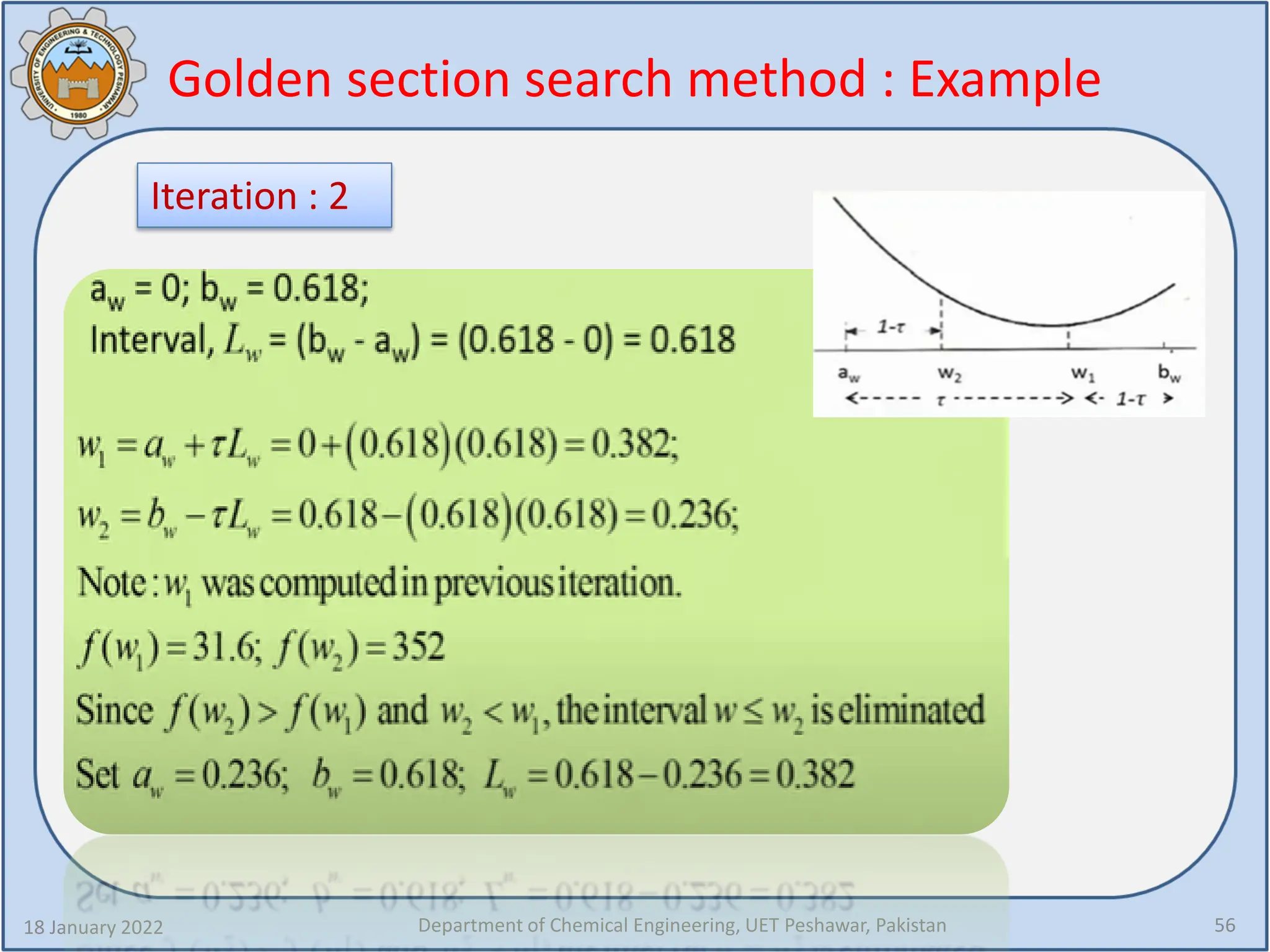
18 January 2022 Department of Chemical Engineering, UET Peshawar, Pakistan 56
Iteration : 2
57.
Golden section searchmethod : Example
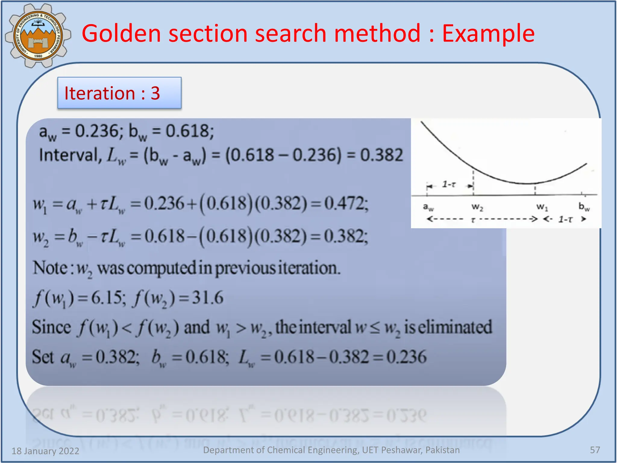
18 January 2022 Department of Chemical Engineering, UET Peshawar, Pakistan 57
Iteration : 3
58.
Unconstrained single variableoptimization
18 January 2022 Department of Chemical Engineering, UET Peshawar, Pakistan 58
General principles of optimization algorithms
Direct Search Methods
Bracketing Methods: Exhaustive search
Region elimination method
Interval halving method
fibonacci method
Golden Search Method
Methods requiring derivatives
Newton-Raphson method
Bisection method
Secant Method
59.
Gradient based searchmethod
18 January 2022 Department of Chemical Engineering, UET Peshawar, Pakistan 59
Gradient based method are more effective and popular . However it
is not easy to obtain derivative information for real life problems.
But when the derivative information is available , these methods are
very fast compared to direct search method.
Analytical derivatives may not always be possible to obtain, in such
cases numerical methods are used to obtain derivatives. There are
various ways like central difference method, forward difference
method, backward difference method etc.
In gradient based methods, the derivative at optimal point is zero,
That is how to obtain a stationary point. So, in these methods the
solution (or roots) of 1st derivatives of the function are find. f ‘(x) = 0,
it also gives us the termination criteria.
60.
Newton Raphson Method
18January 2022 Department of Chemical Engineering, UET Peshawar, Pakistan 60
Isaac-newton
The Newton Raphson method requires that
the function f(x) be twice differentiable .
We start with an initial estimate of the
stationary point x1 – that is the initial
estimate of root of f′(x) = 0.
A linear approximation of the function f′(x) = 0 at the
point x1 is obtained (Through Taylor expansion), and the
point at which the linear approximation is zero is taken as
the next improved approximation of the root of f′(x) = 0 .
61.
Newton Raphson method
18January 2022 Department of Chemical Engineering, UET Peshawar, Pakistan 61
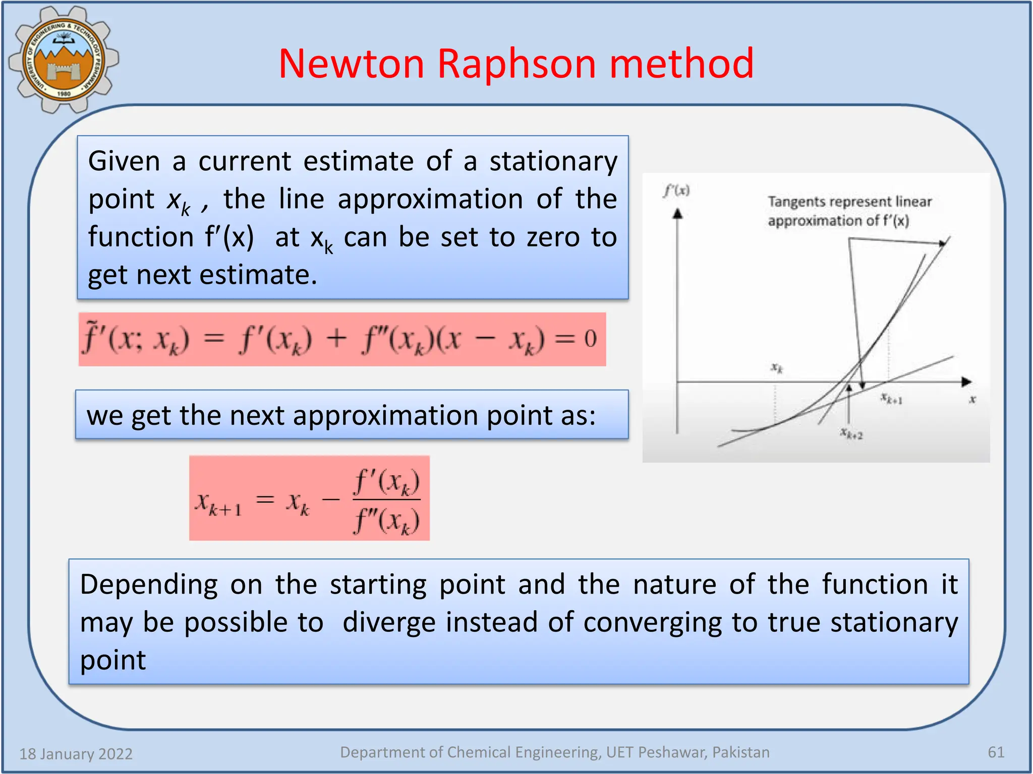
Given a current estimate of a stationary
point xk , the line approximation of the
function f′(x) at xk can be set to zero to
get next estimate.
Depending on the starting point and the nature of the function it
may be possible to diverge instead of converging to true stationary
point
we get the next approximation point as:
62.
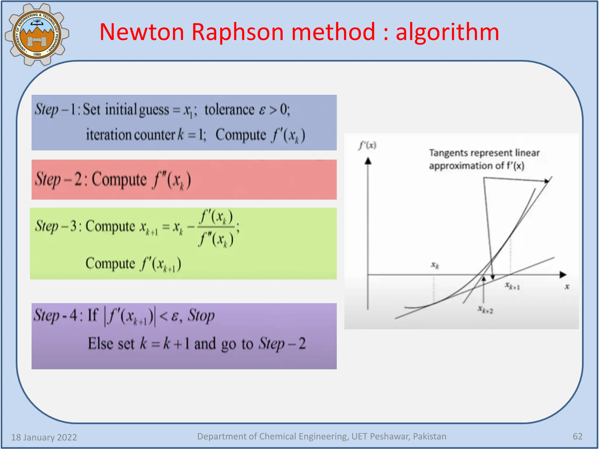
Newton Raphson method: algorithm
18 January 2022 Department of Chemical Engineering, UET Peshawar, Pakistan 62
63.
Newton Raphson method: Numerical
derivatives
18 January 2022 Department of Chemical Engineering, UET Peshawar, Pakistan 63
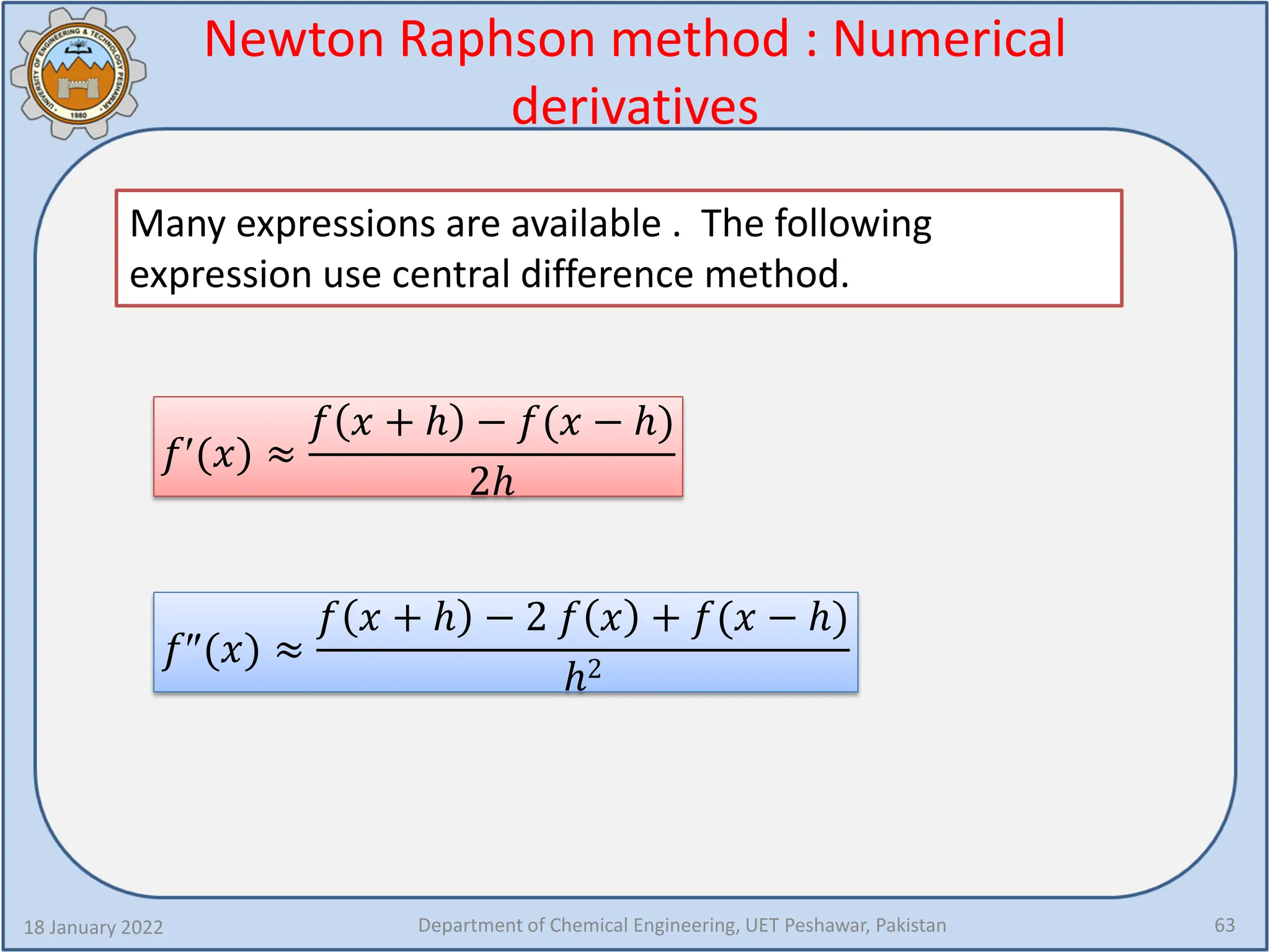
Many expressions are available . The following
expression use central difference method.
𝑓𝑓′(𝑥𝑥) ≈
𝑓𝑓 𝑥𝑥 + ℎ − 𝑓𝑓(𝑥𝑥 − ℎ)
2ℎ
𝑓𝑓″(𝑥𝑥) ≈
𝑓𝑓 𝑥𝑥 + ℎ − 2 𝑓𝑓 𝑥𝑥 + 𝑓𝑓(𝑥𝑥 − ℎ)
ℎ2
64.
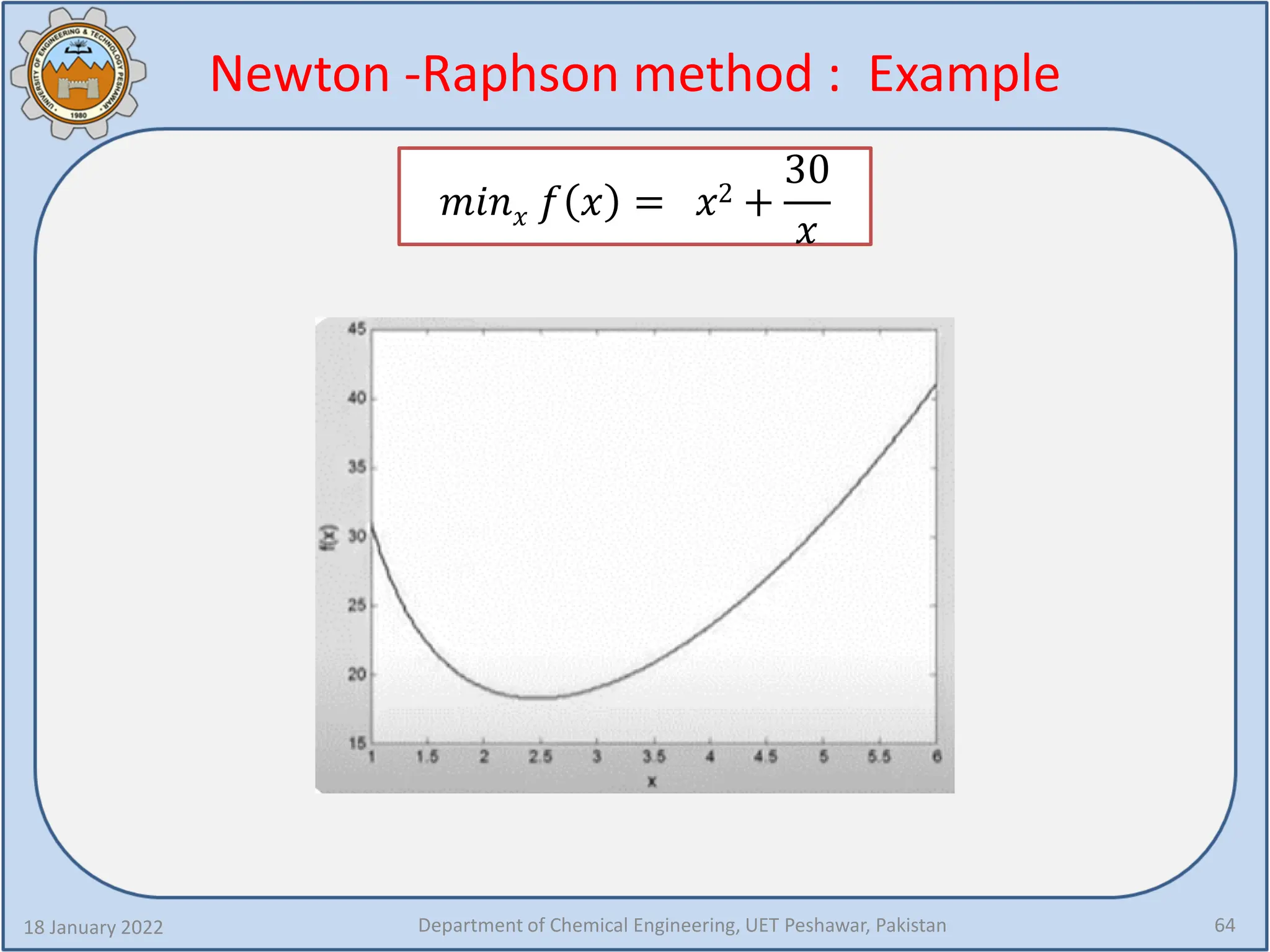
Newton -Raphson method: Example
18 January 2022 Department of Chemical Engineering, UET Peshawar, Pakistan 64
𝑚𝑚𝑚𝑚𝑚𝑚𝑥𝑥 𝑓𝑓 𝑥𝑥 = 𝑥𝑥2 +
30
𝑥𝑥
65.
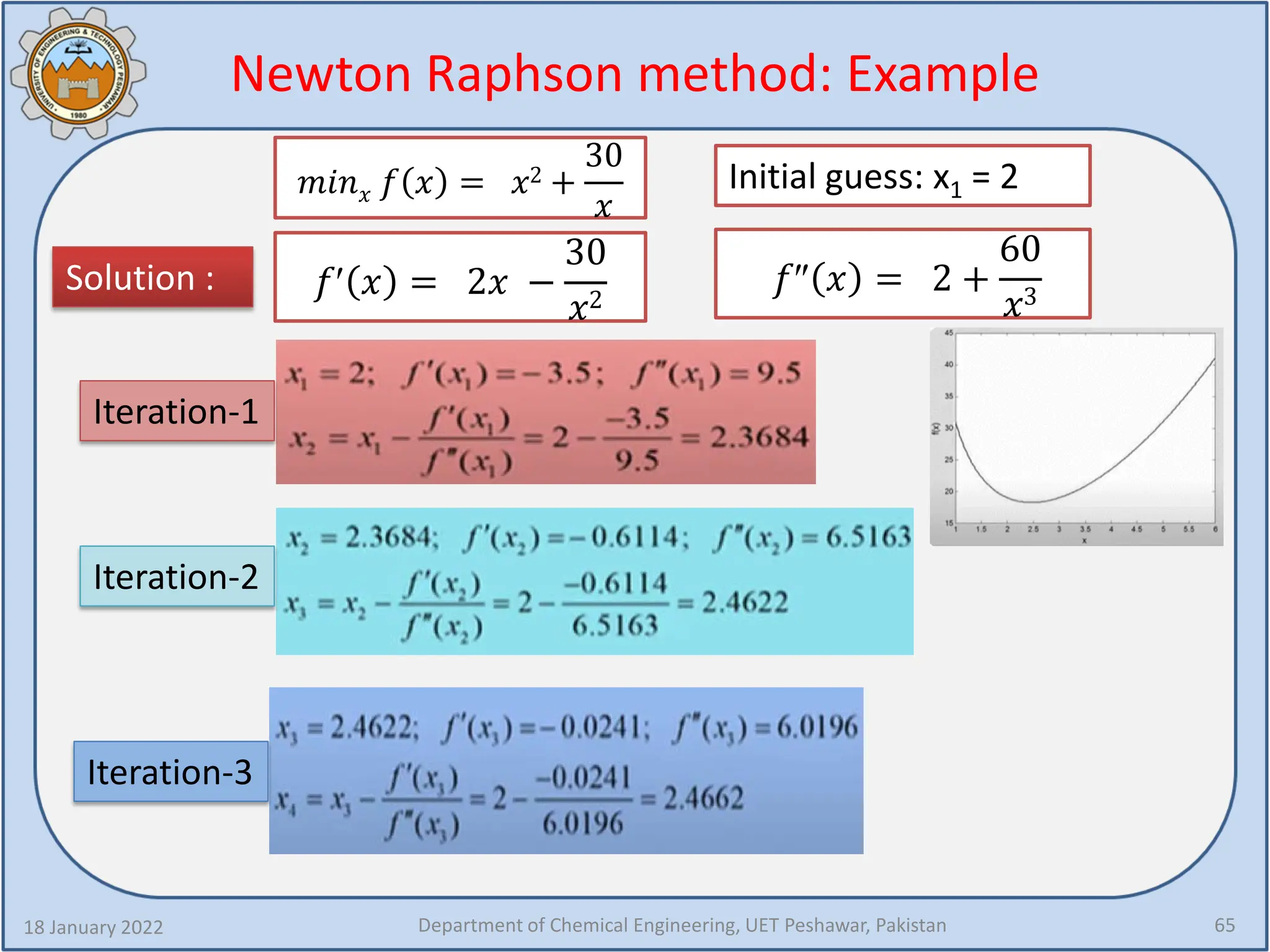
Newton Raphson method:Example
18 January 2022 Department of Chemical Engineering, UET Peshawar, Pakistan 65
𝑚𝑚𝑚𝑚𝑚𝑚𝑥𝑥 𝑓𝑓 𝑥𝑥 = 𝑥𝑥2 +
30
𝑥𝑥
Initial guess: x1 = 2
Solution : 𝑓𝑓″ 𝑥𝑥 = 2 +
60
𝑥𝑥3
𝑓𝑓′ 𝑥𝑥 = 2𝑥𝑥 −
30
𝑥𝑥2
Iteration-1
Iteration-2
Iteration-3
66.
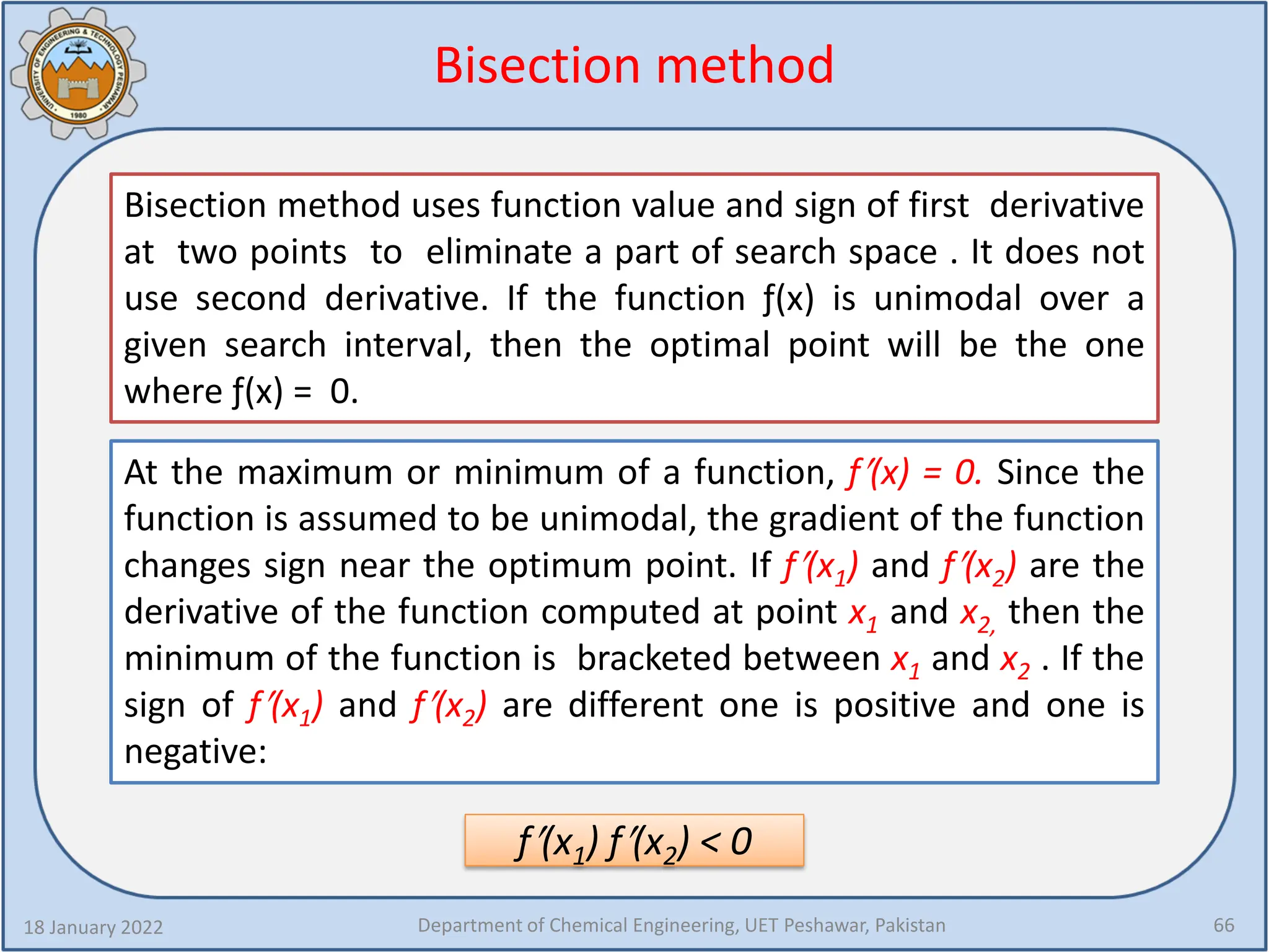
Bisection method
18 January2022 Department of Chemical Engineering, UET Peshawar, Pakistan 66
Bisection method uses function value and sign of first derivative
at two points to eliminate a part of search space . It does not
use second derivative. If the function ƒ(x) is unimodal over a
given search interval, then the optimal point will be the one
where ƒ(x) = 0.
At the maximum or minimum of a function, f′(x) = 0. Since the
function is assumed to be unimodal, the gradient of the function
changes sign near the optimum point. If f′(x1) and f′(x2) are the
derivative of the function computed at point x1 and x2, then the
minimum of the function is bracketed between x1 and x2 . If the
sign of f′(x1) and f′(x2) are different one is positive and one is
negative:
f′(x1) f′(x2) < 0
67.
Bisection method :Algorithm
18 January 2022 Department of Chemical Engineering, UET Peshawar, Pakistan 67
: choose two points [a , b] such that
f′(a) < 0 and f′(b) > 0.
Set x1= a and x2 = b and tolerance ε > 0
compute 𝑧𝑧 =
𝑥𝑥1
+𝑥𝑥2
2
and evaluate f′(z).
: if f′(z) < ε stop.
Else if f′(z) <0 set x1 = z and go to step 2.
Else if f′(z) > 0 set x2 = z and go to step 2.
Consider first derivative sign at mid point.
If derivative is negative, eliminate left half.
If derivative is positive, eliminate right half.
68.
Secant method
18 January2022 Department of Chemical Engineering, UET Peshawar, Pakistan 68
In the bisection method we used only the sign of the derivative to
locate zero of f′(x). In the secant method, both the magnitude and
sign of the derivative is used to locate zero of f′(x).
We start with two points x1 and x2 such that f′(x1) and f′(x2) have
opposite signs : f′(x1) f′(x2) < 0
Next we assume that f′(x) varies linearly between two points x1 and
x2 . A secant line is drawn between these two points . The point z
where the secant line crosses the x-axis is taken as the improved
guess for zero of f′(x) in the next iteration.
One of the point (x1 or x2 ) is then replaced by z using sign of f′(z) and
either [x1, z] or [z, x2] is eliminated . More (or smaller ) than half the
search space may be eliminated .
69.
Secant method :Algorithm
18 January 2022 Department of Chemical Engineering, UET Peshawar, Pakistan 69
Algorithm is the same as bisection method . Note the change is
in the computation of z.
: choose two points [a , b]
such that: f′(a) < 0 and ′ .
Set x1= a and x2 = b and
tolerance ε > 0
compute
𝑧𝑧 = 𝑥𝑥2 =
f′(x2)
f′(x1)−f′(x2)
𝑥𝑥𝑥−𝑥𝑥𝑥
and
evaluate f′(z).
: if f′(z) < ε stop.
Else if f′(z) < 0 set x1 = z and go to step 2.
Else if f′(z) > 0 set x2 = z and go to step 2.
70.
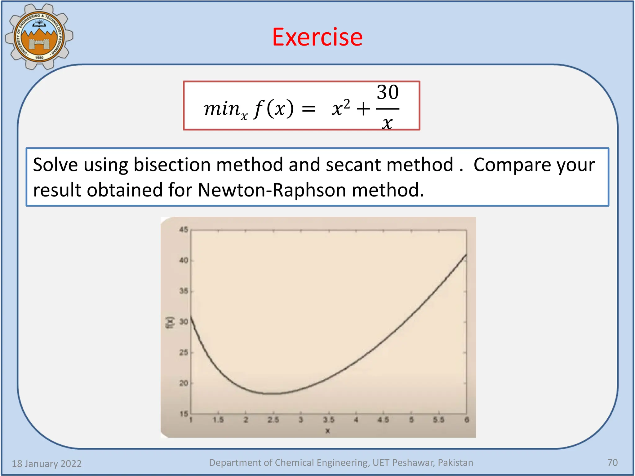
Exercise
18 January 2022Department of Chemical Engineering, UET Peshawar, Pakistan 70
𝑚𝑚𝑚𝑚𝑚𝑚𝑥𝑥 𝑓𝑓 𝑥𝑥 = 𝑥𝑥2 +
30
𝑥𝑥
Solve using bisection method and secant method . Compare your
result obtained for Newton-Raphson method.
71.
18 January 2022Department of Chemical Engineering, UET Peshawar, Pakistan 71
72.
18 January 2022Department of Chemical Engineering, UET Peshawar, Pakistan 72
![Numerical precision
• Solving the first order optimality condition f(x*) = 0 is
equivalent to find the roots of the first derivative of the
function to be minimized.
18 January 2022 Department of Chemical Engineering, UET Peshawar, Pakistan 8
When we use computers it may not always be possible to
find the exact zero due to restriction on mechanic precision .
So we will be satisfied with finding x* that belongs to an
interval [ a, b ] such that the function f satisfies .](https://image.slidesharecdn.com/4-unconstrainedsinglevariableoptimization-methodsandapplication-231030085827-9da5b531/75/4-Unconstrained-Single-Variable-Optimization-Methods-and-Application-pdf-8-2048.jpg)
![Exhaustive search method: Algorithm
18 January 2022 Department of Chemical Engineering, UET Peshawar, Pakistan 17
In the interval (x0 ,xf) the objective function has been
evaluated at n equally spaced point:
X0< X1 <X2 … <Xn <Xf
If the minimum value among the n
function values is xk then the final
interval of uncertainty is [xk-1, xk+1]
with length of :](https://image.slidesharecdn.com/4-unconstrainedsinglevariableoptimization-methodsandapplication-231030085827-9da5b531/75/4-Unconstrained-Single-Variable-Optimization-Methods-and-Application-pdf-17-2048.jpg)
![Exhaustive search method: example 1
18 January 2022 Department of Chemical Engineering, UET Peshawar, Pakistan 18
Find the minimum of 𝑓𝑓 𝑥𝑥 = 𝑥𝑥 𝑥𝑥 − 1.5
in the interval [0,1] to within 10 % of the
exact value .
Plot x vs f(x) for
x=0 to x=1](https://image.slidesharecdn.com/4-unconstrainedsinglevariableoptimization-methodsandapplication-231030085827-9da5b531/75/4-Unconstrained-Single-Variable-Optimization-Methods-and-Application-pdf-18-2048.jpg)
![Exhaustive search method: example 1 cont,d
18 January 2022 Department of Chemical Engineering, UET Peshawar, Pakistan 19
Find the minimum of 𝑓𝑓 𝑥𝑥 = 𝑥𝑥 𝑥𝑥 − 1.5 in the interval
[1,2] to within 10 % of the exact value.
Solution:
If the middle point of the final interval of uncertainty is taken as
the approximate point , the maximum deviation could 1/n+1
times the interval of uncertainty . Thus to find the optimum with
in 10% of the exact value we should have :](https://image.slidesharecdn.com/4-unconstrainedsinglevariableoptimization-methodsandapplication-231030085827-9da5b531/75/4-Unconstrained-Single-Variable-Optimization-Methods-and-Application-pdf-19-2048.jpg)
![Region elimination method : How to place trial
points
18 January 2022 Department of Chemical Engineering, UET Peshawar, Pakistan 27
Fundamental rules of region elimination:
Note that depending on function value we will delete [a, x1]
,[x2,b] or both. In order to reduce interval of uncertainty ,we
would like to maximize the length of [a, x1] or ,[x2,b] .To maximize
both we should place x1 and x2 symmetrically in the interval
[a,b].](https://image.slidesharecdn.com/4-unconstrainedsinglevariableoptimization-methodsandapplication-231030085827-9da5b531/75/4-Unconstrained-Single-Variable-Optimization-Methods-and-Application-pdf-27-2048.jpg)
![Region elimination method : Dichotomous search
18 January 2022 Department of Chemical Engineering, UET Peshawar, Pakistan 28
Let the optimum lie between [a,b]. The dichotomous
method first compute the mid point a+b//2 and then move
slightly to either side of the mid-point to compute two test
points : a+b/2 +
� ε.
Based on the function values and
unimodality assumptions, the
interval is updated by eliminating
one part and the procedure
continuous until the optimal
solution is contained in a small
interval.
This method is also known as method of bisecting.](https://image.slidesharecdn.com/4-unconstrainedsinglevariableoptimization-methodsandapplication-231030085827-9da5b531/75/4-Unconstrained-Single-Variable-Optimization-Methods-and-Application-pdf-28-2048.jpg)
![Region elimination: interval halving method
18 January 2022 Department of Chemical Engineering, UET Peshawar, Pakistan 31
Once the optimum has been bracketed, region elimination
method give us a more refined estimate of the optimum by
eliminating certain amount of subinterval at each step.
Internal halving method
eliminate exactly one-half of
the interval at each stage
by considering three equally
spaced trail points. These
three points divide the
interval [a,b] into 4 equal
regions.](https://image.slidesharecdn.com/4-unconstrainedsinglevariableoptimization-methodsandapplication-231030085827-9da5b531/75/4-Unconstrained-Single-Variable-Optimization-Methods-and-Application-pdf-31-2048.jpg)
![Region elimination interval halving method:
Algorithm
18 January 2022 Department of Chemical Engineering, UET Peshawar, Pakistan 33
Step-3: If f(x1) < f(xm), set xm = b; and x1 = xm; go to step-5;
Else go step-2, step, 4
Step-4: If f(x2) < f(xm), set xm = a; and x2 = xm; go to step-5;
Else set x1 = a; x2 = b; go to step-5
Step-5: Evaluate L = (b - a), if I L I < ɛ, stop;
Else go to step-2
Step-2: Set x1 = a + L/4, x2 = b – L/4. Evaluate f(x1), f(x2)
Step-1: Given x* Є [a, b], L0 = L = (b-a), ɛ > 0
Let xm = (a + b)/2; Evaluate f(xm)](https://image.slidesharecdn.com/4-unconstrainedsinglevariableoptimization-methodsandapplication-231030085827-9da5b531/75/4-Unconstrained-Single-Variable-Optimization-Methods-and-Application-pdf-33-2048.jpg)
![Interval halving method example
Find the minimum of 𝑓𝑓 𝑥𝑥 = 𝑥𝑥 𝑥𝑥 − 1.5 in the interval [0,1] to
within 10 % of the exact value.
Solution:
If the middle point of the final interval of uncertainty is taken as
the optimum point , the specified accuracy can be achieved if
18 January 2022 Department of Chemical Engineering, UET Peshawar, Pakistan 35
and also,](https://image.slidesharecdn.com/4-unconstrainedsinglevariableoptimization-methodsandapplication-231030085827-9da5b531/75/4-Unconstrained-Single-Variable-Optimization-Methods-and-Application-pdf-35-2048.jpg)
![Interval halving method Homework
Consider 𝑓𝑓 𝑥𝑥 = 100 − 𝑥𝑥2 .
Find xopt by interval halving method. Take x=[60,150].
Note xopt = 100.
Perform 3 iteration and see that the mid point of the interval
after 3 iterations is already 99.375.
18 January 2022 Department of Chemical Engineering, UET Peshawar, Pakistan 38](https://image.slidesharecdn.com/4-unconstrainedsinglevariableoptimization-methodsandapplication-231030085827-9da5b531/75/4-Unconstrained-Single-Variable-Optimization-Methods-and-Application-pdf-38-2048.jpg)
![Region elimination : Fibonacci search method
18 January 2022 Department of Chemical Engineering, UET Peshawar, Pakistan 40
Fibonacci search methods use the sequence of
Fibonacci numbers [Fn], to reduce the interval of
uncertainty. These numbers are defined as:
𝐹𝐹0 = 𝐹𝐹1 = 1
𝐹𝐹𝑛𝑛 = 𝐹𝐹 𝑛𝑛 − 1 +
𝐹𝐹𝑛𝑛 − 2,
𝑛𝑛 = 2, 3, 4 …
Each number after the first two represent the sum of the
proceeding two.
First few Fibonacci numbers are 1, 1, 2, 3, 5, 8, 13, 21, 34, 55, 89,…](https://image.slidesharecdn.com/4-unconstrainedsinglevariableoptimization-methodsandapplication-231030085827-9da5b531/75/4-Unconstrained-Single-Variable-Optimization-Methods-and-Application-pdf-40-2048.jpg)
![Fibonacci search method: example
18 January 2022 Department of Chemical Engineering, UET Peshawar, Pakistan 45
Using Fibonacci search method, minimize the following
function in the interval x = [1, 6]. Perform 3 iteration (n=3).
𝑚𝑚𝑚𝑚𝑚𝑚𝑥𝑥 𝑓𝑓 𝑥𝑥 = 𝑥𝑥2 +
30
𝑥𝑥](https://image.slidesharecdn.com/4-unconstrainedsinglevariableoptimization-methodsandapplication-231030085827-9da5b531/75/4-Unconstrained-Single-Variable-Optimization-Methods-and-Application-pdf-45-2048.jpg)
![Example cont,d
18 January 2022 Department of Chemical Engineering, UET Peshawar, Pakistan 48
Iteration 2, step 1:
Second iteration complete
Iteration 2, step 3:
Minimum is bracketed between [2,3] . In
actual practice we should consider higher
value of n and proceed as shown.](https://image.slidesharecdn.com/4-unconstrainedsinglevariableoptimization-methodsandapplication-231030085827-9da5b531/75/4-Unconstrained-Single-Variable-Optimization-Methods-and-Application-pdf-48-2048.jpg)
![Golden section search method : Algorithm
18 January 2022 Department of Chemical Engineering, UET Peshawar, Pakistan 52
τ 1 − τ
1. Start with a unit interval of convenience. Thus the given interval may be
scaled up to [0,1]. .
2. Place two trail points a friction τ from either end.
3. Suppose RHS interval is eliminated he remaining subinterval has length τ
and it has an old trial point located interior to it at a distance (1- τ ) from
the left end point.
4. Each subsequent iteration will eliminate (1- τ ) of the remaining interval
.thus after n function evaluation the interval remaining will be ( τn-1 )](https://image.slidesharecdn.com/4-unconstrainedsinglevariableoptimization-methodsandapplication-231030085827-9da5b531/75/4-Unconstrained-Single-Variable-Optimization-Methods-and-Application-pdf-52-2048.jpg)
![Golden section search method : Example
18 January 2022 Department of Chemical Engineering, UET Peshawar, Pakistan 54
minx f x = 100 − x 2 60 ≤ x ≤ 150
Solution:
Let us first scale the interval [60,150] to [0,1] and
reformulate the problem:
𝑤𝑤 =
𝑥𝑥−60
150−60
=
𝑥𝑥−60
90
minx f w = 40 − 90𝑤𝑤 2, 0 ≤ w ≤ 1](https://image.slidesharecdn.com/4-unconstrainedsinglevariableoptimization-methodsandapplication-231030085827-9da5b531/75/4-Unconstrained-Single-Variable-Optimization-Methods-and-Application-pdf-54-2048.jpg)
![Bisection method : Algorithm
18 January 2022 Department of Chemical Engineering, UET Peshawar, Pakistan 67
: choose two points [a , b] such that
f′(a) < 0 and f′(b) > 0.
Set x1= a and x2 = b and tolerance ε > 0
compute 𝑧𝑧 =
𝑥𝑥1
+𝑥𝑥2
2
and evaluate f′(z).
: if f′(z) < ε stop.
Else if f′(z) <0 set x1 = z and go to step 2.
Else if f′(z) > 0 set x2 = z and go to step 2.
Consider first derivative sign at mid point.
If derivative is negative, eliminate left half.
If derivative is positive, eliminate right half.](https://image.slidesharecdn.com/4-unconstrainedsinglevariableoptimization-methodsandapplication-231030085827-9da5b531/75/4-Unconstrained-Single-Variable-Optimization-Methods-and-Application-pdf-67-2048.jpg)
![Secant method
18 January 2022 Department of Chemical Engineering, UET Peshawar, Pakistan 68
In the bisection method we used only the sign of the derivative to
locate zero of f′(x). In the secant method, both the magnitude and
sign of the derivative is used to locate zero of f′(x).
We start with two points x1 and x2 such that f′(x1) and f′(x2) have
opposite signs : f′(x1) f′(x2) < 0
Next we assume that f′(x) varies linearly between two points x1 and
x2 . A secant line is drawn between these two points . The point z
where the secant line crosses the x-axis is taken as the improved
guess for zero of f′(x) in the next iteration.
One of the point (x1 or x2 ) is then replaced by z using sign of f′(z) and
either [x1, z] or [z, x2] is eliminated . More (or smaller ) than half the
search space may be eliminated .](https://image.slidesharecdn.com/4-unconstrainedsinglevariableoptimization-methodsandapplication-231030085827-9da5b531/75/4-Unconstrained-Single-Variable-Optimization-Methods-and-Application-pdf-68-2048.jpg)
![Secant method : Algorithm
18 January 2022 Department of Chemical Engineering, UET Peshawar, Pakistan 69
Algorithm is the same as bisection method . Note the change is
in the computation of z.
: choose two points [a , b]
such that: f′(a) < 0 and ′ .
Set x1= a and x2 = b and
tolerance ε > 0
compute
𝑧𝑧 = 𝑥𝑥2 =
f′(x2)
f′(x1)−f′(x2)
𝑥𝑥𝑥−𝑥𝑥𝑥
and
evaluate f′(z).
: if f′(z) < ε stop.
Else if f′(z) < 0 set x1 = z and go to step 2.
Else if f′(z) > 0 set x2 = z and go to step 2.](https://image.slidesharecdn.com/4-unconstrainedsinglevariableoptimization-methodsandapplication-231030085827-9da5b531/75/4-Unconstrained-Single-Variable-Optimization-Methods-and-Application-pdf-69-2048.jpg)


![Numerical precision
• Solving the first order optimality condition f(x*) = 0 is
equivalent to find the roots of the first derivative of the
function to be minimized.
18 January 2022 Department of Chemical Engineering, UET Peshawar, Pakistan 8
When we use computers it may not always be possible to
find the exact zero due to restriction on mechanic precision .
So we will be satisfied with finding x* that belongs to an
interval [ a, b ] such that the function f satisfies .](https://crownmelresort.com/image.slidesharecdn.com/4-unconstrainedsinglevariableoptimization-methodsandapplication-231030085827-9da5b531/75/4-Unconstrained-Single-Variable-Optimization-Methods-and-Application-pdf-8-2048.jpg)


![Exhaustive search method: Algorithm
18 January 2022 Department of Chemical Engineering, UET Peshawar, Pakistan 17
In the interval (x0 ,xf) the objective function has been
evaluated at n equally spaced point:
X0< X1 <X2 … <Xn <Xf
If the minimum value among the n
function values is xk then the final
interval of uncertainty is [xk-1, xk+1]
with length of :](https://crownmelresort.com/image.slidesharecdn.com/4-unconstrainedsinglevariableoptimization-methodsandapplication-231030085827-9da5b531/75/4-Unconstrained-Single-Variable-Optimization-Methods-and-Application-pdf-17-2048.jpg)
![Exhaustive search method: example 1
18 January 2022 Department of Chemical Engineering, UET Peshawar, Pakistan 18
Find the minimum of 𝑓𝑓 𝑥𝑥 = 𝑥𝑥 𝑥𝑥 − 1.5
in the interval [0,1] to within 10 % of the
exact value .
Plot x vs f(x) for
x=0 to x=1](https://crownmelresort.com/image.slidesharecdn.com/4-unconstrainedsinglevariableoptimization-methodsandapplication-231030085827-9da5b531/75/4-Unconstrained-Single-Variable-Optimization-Methods-and-Application-pdf-18-2048.jpg)
![Exhaustive search method: example 1 cont,d
18 January 2022 Department of Chemical Engineering, UET Peshawar, Pakistan 19
Find the minimum of 𝑓𝑓 𝑥𝑥 = 𝑥𝑥 𝑥𝑥 − 1.5 in the interval
[1,2] to within 10 % of the exact value.
Solution:
If the middle point of the final interval of uncertainty is taken as
the approximate point , the maximum deviation could 1/n+1
times the interval of uncertainty . Thus to find the optimum with
in 10% of the exact value we should have :](https://crownmelresort.com/image.slidesharecdn.com/4-unconstrainedsinglevariableoptimization-methodsandapplication-231030085827-9da5b531/75/4-Unconstrained-Single-Variable-Optimization-Methods-and-Application-pdf-19-2048.jpg)


![Region elimination method : How to place trial
points
18 January 2022 Department of Chemical Engineering, UET Peshawar, Pakistan 27
Fundamental rules of region elimination:
Note that depending on function value we will delete [a, x1]
,[x2,b] or both. In order to reduce interval of uncertainty ,we
would like to maximize the length of [a, x1] or ,[x2,b] .To maximize
both we should place x1 and x2 symmetrically in the interval
[a,b].](https://crownmelresort.com/image.slidesharecdn.com/4-unconstrainedsinglevariableoptimization-methodsandapplication-231030085827-9da5b531/75/4-Unconstrained-Single-Variable-Optimization-Methods-and-Application-pdf-27-2048.jpg)
![Region elimination method : Dichotomous search
18 January 2022 Department of Chemical Engineering, UET Peshawar, Pakistan 28
Let the optimum lie between [a,b]. The dichotomous
method first compute the mid point a+b//2 and then move
slightly to either side of the mid-point to compute two test
points : a+b/2 +
� ε.
Based on the function values and
unimodality assumptions, the
interval is updated by eliminating
one part and the procedure
continuous until the optimal
solution is contained in a small
interval.
This method is also known as method of bisecting.](https://crownmelresort.com/image.slidesharecdn.com/4-unconstrainedsinglevariableoptimization-methodsandapplication-231030085827-9da5b531/75/4-Unconstrained-Single-Variable-Optimization-Methods-and-Application-pdf-28-2048.jpg)


![Region elimination: interval halving method
18 January 2022 Department of Chemical Engineering, UET Peshawar, Pakistan 31
Once the optimum has been bracketed, region elimination
method give us a more refined estimate of the optimum by
eliminating certain amount of subinterval at each step.
Internal halving method
eliminate exactly one-half of
the interval at each stage
by considering three equally
spaced trail points. These
three points divide the
interval [a,b] into 4 equal
regions.](https://crownmelresort.com/image.slidesharecdn.com/4-unconstrainedsinglevariableoptimization-methodsandapplication-231030085827-9da5b531/75/4-Unconstrained-Single-Variable-Optimization-Methods-and-Application-pdf-31-2048.jpg)

![Region elimination interval halving method:
Algorithm
18 January 2022 Department of Chemical Engineering, UET Peshawar, Pakistan 33
Step-3: If f(x1) < f(xm), set xm = b; and x1 = xm; go to step-5;
Else go step-2, step, 4
Step-4: If f(x2) < f(xm), set xm = a; and x2 = xm; go to step-5;
Else set x1 = a; x2 = b; go to step-5
Step-5: Evaluate L = (b - a), if I L I < ɛ, stop;
Else go to step-2
Step-2: Set x1 = a + L/4, x2 = b – L/4. Evaluate f(x1), f(x2)
Step-1: Given x* Є [a, b], L0 = L = (b-a), ɛ > 0
Let xm = (a + b)/2; Evaluate f(xm)](https://crownmelresort.com/image.slidesharecdn.com/4-unconstrainedsinglevariableoptimization-methodsandapplication-231030085827-9da5b531/75/4-Unconstrained-Single-Variable-Optimization-Methods-and-Application-pdf-33-2048.jpg)

![Interval halving method example
Find the minimum of 𝑓𝑓 𝑥𝑥 = 𝑥𝑥 𝑥𝑥 − 1.5 in the interval [0,1] to
within 10 % of the exact value.
Solution:
If the middle point of the final interval of uncertainty is taken as
the optimum point , the specified accuracy can be achieved if
18 January 2022 Department of Chemical Engineering, UET Peshawar, Pakistan 35
and also,](https://crownmelresort.com/image.slidesharecdn.com/4-unconstrainedsinglevariableoptimization-methodsandapplication-231030085827-9da5b531/75/4-Unconstrained-Single-Variable-Optimization-Methods-and-Application-pdf-35-2048.jpg)


![Interval halving method Homework
Consider 𝑓𝑓 𝑥𝑥 = 100 − 𝑥𝑥2 .
Find xopt by interval halving method. Take x=[60,150].
Note xopt = 100.
Perform 3 iteration and see that the mid point of the interval
after 3 iterations is already 99.375.
18 January 2022 Department of Chemical Engineering, UET Peshawar, Pakistan 38](https://crownmelresort.com/image.slidesharecdn.com/4-unconstrainedsinglevariableoptimization-methodsandapplication-231030085827-9da5b531/75/4-Unconstrained-Single-Variable-Optimization-Methods-and-Application-pdf-38-2048.jpg)

![Region elimination : Fibonacci search method
18 January 2022 Department of Chemical Engineering, UET Peshawar, Pakistan 40
Fibonacci search methods use the sequence of
Fibonacci numbers [Fn], to reduce the interval of
uncertainty. These numbers are defined as:
𝐹𝐹0 = 𝐹𝐹1 = 1
𝐹𝐹𝑛𝑛 = 𝐹𝐹 𝑛𝑛 − 1 +
𝐹𝐹𝑛𝑛 − 2,
𝑛𝑛 = 2, 3, 4 …
Each number after the first two represent the sum of the
proceeding two.
First few Fibonacci numbers are 1, 1, 2, 3, 5, 8, 13, 21, 34, 55, 89,…](https://crownmelresort.com/image.slidesharecdn.com/4-unconstrainedsinglevariableoptimization-methodsandapplication-231030085827-9da5b531/75/4-Unconstrained-Single-Variable-Optimization-Methods-and-Application-pdf-40-2048.jpg)


![Fibonacci search method: example
18 January 2022 Department of Chemical Engineering, UET Peshawar, Pakistan 45
Using Fibonacci search method, minimize the following
function in the interval x = [1, 6]. Perform 3 iteration (n=3).
𝑚𝑚𝑚𝑚𝑚𝑚𝑥𝑥 𝑓𝑓 𝑥𝑥 = 𝑥𝑥2 +
30
𝑥𝑥](https://crownmelresort.com/image.slidesharecdn.com/4-unconstrainedsinglevariableoptimization-methodsandapplication-231030085827-9da5b531/75/4-Unconstrained-Single-Variable-Optimization-Methods-and-Application-pdf-45-2048.jpg)


![Example cont,d
18 January 2022 Department of Chemical Engineering, UET Peshawar, Pakistan 48
Iteration 2, step 1:
Second iteration complete
Iteration 2, step 3:
Minimum is bracketed between [2,3] . In
actual practice we should consider higher
value of n and proceed as shown.](https://crownmelresort.com/image.slidesharecdn.com/4-unconstrainedsinglevariableoptimization-methodsandapplication-231030085827-9da5b531/75/4-Unconstrained-Single-Variable-Optimization-Methods-and-Application-pdf-48-2048.jpg)


![Golden section search method : Algorithm
18 January 2022 Department of Chemical Engineering, UET Peshawar, Pakistan 52
τ 1 − τ
1. Start with a unit interval of convenience. Thus the given interval may be
scaled up to [0,1]. .
2. Place two trail points a friction τ from either end.
3. Suppose RHS interval is eliminated he remaining subinterval has length τ
and it has an old trial point located interior to it at a distance (1- τ ) from
the left end point.
4. Each subsequent iteration will eliminate (1- τ ) of the remaining interval
.thus after n function evaluation the interval remaining will be ( τn-1 )](https://crownmelresort.com/image.slidesharecdn.com/4-unconstrainedsinglevariableoptimization-methodsandapplication-231030085827-9da5b531/75/4-Unconstrained-Single-Variable-Optimization-Methods-and-Application-pdf-52-2048.jpg)

![Golden section search method : Example
18 January 2022 Department of Chemical Engineering, UET Peshawar, Pakistan 54
minx f x = 100 − x 2 60 ≤ x ≤ 150
Solution:
Let us first scale the interval [60,150] to [0,1] and
reformulate the problem:
𝑤𝑤 =
𝑥𝑥−60
150−60
=
𝑥𝑥−60
90
minx f w = 40 − 90𝑤𝑤 2, 0 ≤ w ≤ 1](https://crownmelresort.com/image.slidesharecdn.com/4-unconstrainedsinglevariableoptimization-methodsandapplication-231030085827-9da5b531/75/4-Unconstrained-Single-Variable-Optimization-Methods-and-Application-pdf-54-2048.jpg)


![Bisection method : Algorithm
18 January 2022 Department of Chemical Engineering, UET Peshawar, Pakistan 67
: choose two points [a , b] such that
f′(a) < 0 and f′(b) > 0.
Set x1= a and x2 = b and tolerance ε > 0
compute 𝑧𝑧 =
𝑥𝑥1
+𝑥𝑥2
2
and evaluate f′(z).
: if f′(z) < ε stop.
Else if f′(z) <0 set x1 = z and go to step 2.
Else if f′(z) > 0 set x2 = z and go to step 2.
Consider first derivative sign at mid point.
If derivative is negative, eliminate left half.
If derivative is positive, eliminate right half.](https://crownmelresort.com/image.slidesharecdn.com/4-unconstrainedsinglevariableoptimization-methodsandapplication-231030085827-9da5b531/75/4-Unconstrained-Single-Variable-Optimization-Methods-and-Application-pdf-67-2048.jpg)
![Secant method
18 January 2022 Department of Chemical Engineering, UET Peshawar, Pakistan 68
In the bisection method we used only the sign of the derivative to
locate zero of f′(x). In the secant method, both the magnitude and
sign of the derivative is used to locate zero of f′(x).
We start with two points x1 and x2 such that f′(x1) and f′(x2) have
opposite signs : f′(x1) f′(x2) < 0
Next we assume that f′(x) varies linearly between two points x1 and
x2 . A secant line is drawn between these two points . The point z
where the secant line crosses the x-axis is taken as the improved
guess for zero of f′(x) in the next iteration.
One of the point (x1 or x2 ) is then replaced by z using sign of f′(z) and
either [x1, z] or [z, x2] is eliminated . More (or smaller ) than half the
search space may be eliminated .](https://crownmelresort.com/image.slidesharecdn.com/4-unconstrainedsinglevariableoptimization-methodsandapplication-231030085827-9da5b531/75/4-Unconstrained-Single-Variable-Optimization-Methods-and-Application-pdf-68-2048.jpg)
![Secant method : Algorithm
18 January 2022 Department of Chemical Engineering, UET Peshawar, Pakistan 69
Algorithm is the same as bisection method . Note the change is
in the computation of z.
: choose two points [a , b]
such that: f′(a) < 0 and ′ .
Set x1= a and x2 = b and
tolerance ε > 0
compute
𝑧𝑧 = 𝑥𝑥2 =
f′(x2)
f′(x1)−f′(x2)
𝑥𝑥𝑥−𝑥𝑥𝑥
and
evaluate f′(z).
: if f′(z) < ε stop.
Else if f′(z) < 0 set x1 = z and go to step 2.
Else if f′(z) > 0 set x2 = z and go to step 2.](https://crownmelresort.com/image.slidesharecdn.com/4-unconstrainedsinglevariableoptimization-methodsandapplication-231030085827-9da5b531/75/4-Unconstrained-Single-Variable-Optimization-Methods-and-Application-pdf-69-2048.jpg)