Download as PDF, PPTX


![Greedy Search: Tree Search
Start
A 75
118
[329] 140 [374] B
C
[253] E](https://image.slidesharecdn.com/16890unit2heuristicsearchtechniques-130225201019-phpapp01/75/16890-unit-2-heuristic-search-techniques-30-2048.jpg)
![Greedy Search: Tree Search
Start
A 75
118
[329] 140 [374] B
C
[253] E
80 99
[193] [178]
G F
[366] A](https://image.slidesharecdn.com/16890unit2heuristicsearchtechniques-130225201019-phpapp01/75/16890-unit-2-heuristic-search-techniques-31-2048.jpg)
![Greedy Search: Tree Search
Start
A 75
118
[329] 140 [374] B
C
[253] E
80 99
[193] [178]
G F
[366] A
211
[253] I [0]
E
Goal](https://image.slidesharecdn.com/16890unit2heuristicsearchtechniques-130225201019-phpapp01/75/16890-unit-2-heuristic-search-techniques-32-2048.jpg)
![Greedy Search: Tree Search
Start
A 75
118
[329] 140 [374] B
C
[253] E
80 99
[193] [178]
G F
[366] A
211
[253] I [0]
E
Goal
Path cost(A-E-F-I) = 253 + 178 + 0 = 431
dist(A-E-F-I) = 140 + 99 + 211 = 450](https://image.slidesharecdn.com/16890unit2heuristicsearchtechniques-130225201019-phpapp01/75/16890-unit-2-heuristic-search-techniques-33-2048.jpg)
![Greedy Search: Tree Search
Start
A 75
118
[250] 140 [374] B
C
[253] E](https://image.slidesharecdn.com/16890unit2heuristicsearchtechniques-130225201019-phpapp01/75/16890-unit-2-heuristic-search-techniques-37-2048.jpg)
![Greedy Search: Tree Search
Start
A 75
118
[250] 140 [374] B
C
[253] E
111
[244] D](https://image.slidesharecdn.com/16890unit2heuristicsearchtechniques-130225201019-phpapp01/75/16890-unit-2-heuristic-search-techniques-38-2048.jpg)
![Greedy Search: Tree Search
Start
A 75
118
[250] 140 [374] B
C
[253] E
111
[244] D
Infinite Branch !
[250] C](https://image.slidesharecdn.com/16890unit2heuristicsearchtechniques-130225201019-phpapp01/75/16890-unit-2-heuristic-search-techniques-39-2048.jpg)
![Greedy Search: Tree Search
Start
A 75
118
[250] 140 [374] B
C
[253] E
111
[244] D
Infinite Branch !
[250] C
[244] D](https://image.slidesharecdn.com/16890unit2heuristicsearchtechniques-130225201019-phpapp01/75/16890-unit-2-heuristic-search-techniques-40-2048.jpg)
![Greedy Search: Tree Search
Start
A 75
118
[250] 140 [374] B
C
[253] E
111
[244] D
Infinite Branch !
[250] C
[244] D](https://image.slidesharecdn.com/16890unit2heuristicsearchtechniques-130225201019-phpapp01/75/16890-unit-2-heuristic-search-techniques-41-2048.jpg)
![Uniform Cost Search (UCS)
5 2
[5] [2]
1 4 1 7
[6] [3] [9]
[9]
Goal state
4 5
[x] = g(n) [7] [8]
path cost of node n](https://image.slidesharecdn.com/16890unit2heuristicsearchtechniques-130225201019-phpapp01/75/16890-unit-2-heuristic-search-techniques-44-2048.jpg)
![Uniform Cost Search (UCS)
5 2
[5] [2]](https://image.slidesharecdn.com/16890unit2heuristicsearchtechniques-130225201019-phpapp01/75/16890-unit-2-heuristic-search-techniques-45-2048.jpg)
![Uniform Cost Search (UCS)
5 2
[5] [2]
1 7
[3] [9]](https://image.slidesharecdn.com/16890unit2heuristicsearchtechniques-130225201019-phpapp01/75/16890-unit-2-heuristic-search-techniques-46-2048.jpg)
![Uniform Cost Search (UCS)
5 2
[5] [2]
1 7
[3] [9]
4 5
[7] [8]](https://image.slidesharecdn.com/16890unit2heuristicsearchtechniques-130225201019-phpapp01/75/16890-unit-2-heuristic-search-techniques-47-2048.jpg)
![Uniform Cost Search (UCS)
5 2
[5] [2]
1 4 1 7
[6] [3] [9]
[9]
4 5
[7] [8]](https://image.slidesharecdn.com/16890unit2heuristicsearchtechniques-130225201019-phpapp01/75/16890-unit-2-heuristic-search-techniques-48-2048.jpg)
![Uniform Cost Search (UCS)
5 2
[5] [2]
Goal state
path cost 1 4 1 7
g(n)=[6]
[3] [9]
[9]
4 5
[7] [8]](https://image.slidesharecdn.com/16890unit2heuristicsearchtechniques-130225201019-phpapp01/75/16890-unit-2-heuristic-search-techniques-49-2048.jpg)
![Uniform Cost Search (UCS)
5 2
[5] [2]
1 4 1 7
[6] [3] [9]
[9]
4 5
[7] [8]](https://image.slidesharecdn.com/16890unit2heuristicsearchtechniques-130225201019-phpapp01/75/16890-unit-2-heuristic-search-techniques-50-2048.jpg)


![A* Search: Tree Search
A Start
118 75
140
[447] C E [393] B [449]](https://image.slidesharecdn.com/16890unit2heuristicsearchtechniques-130225201019-phpapp01/75/16890-unit-2-heuristic-search-techniques-61-2048.jpg)
![A* Search: Tree Search
A Start
118 75
140
[447] C E [393] B [449]
80 99
[413] G F [417]](https://image.slidesharecdn.com/16890unit2heuristicsearchtechniques-130225201019-phpapp01/75/16890-unit-2-heuristic-search-techniques-62-2048.jpg)
![A* Search: Tree Search
A Start
118 75
140
[447] C E [393] B [449]
80 99
[413] G F [417]
97
[415] H](https://image.slidesharecdn.com/16890unit2heuristicsearchtechniques-130225201019-phpapp01/75/16890-unit-2-heuristic-search-techniques-63-2048.jpg)
![A* Search: Tree Search
A Start
118 75
140
[447] C E [393] B [449]
80 99
[413] G F [417]
97
[415] H
101
Goal I [418]](https://image.slidesharecdn.com/16890unit2heuristicsearchtechniques-130225201019-phpapp01/75/16890-unit-2-heuristic-search-techniques-64-2048.jpg)
![A* Search: Tree Search
A Start
118 75
140
[447] C E [393] B [449]
80 99
[413] G F [417]
97
[415] H I [450]
101
Goal I [418]](https://image.slidesharecdn.com/16890unit2heuristicsearchtechniques-130225201019-phpapp01/75/16890-unit-2-heuristic-search-techniques-65-2048.jpg)
![A* Search: Tree Search
A Start
118 75
140
[447] C E [393] B [449]
80 99
[413] G F [417]
97
[415] H I [450]
101
Goal I [418]](https://image.slidesharecdn.com/16890unit2heuristicsearchtechniques-130225201019-phpapp01/75/16890-unit-2-heuristic-search-techniques-66-2048.jpg)
![A* Search: Tree Search
A Start
118 75
140
[447] C E [393] B [449]
80 99
[413] G F [417]
97
[415] H I [450]
101
Goal I [418]](https://image.slidesharecdn.com/16890unit2heuristicsearchtechniques-130225201019-phpapp01/75/16890-unit-2-heuristic-search-techniques-67-2048.jpg)
![A* Search: Tree Search
A Start
118 75
140
[447] C E [393] B [449]](https://image.slidesharecdn.com/16890unit2heuristicsearchtechniques-130225201019-phpapp01/75/16890-unit-2-heuristic-search-techniques-71-2048.jpg)
![A* Search: Tree Search
A Start
118 75
140
[447] C E [393] B [449]
80 99
[413] G F [417]](https://image.slidesharecdn.com/16890unit2heuristicsearchtechniques-130225201019-phpapp01/75/16890-unit-2-heuristic-search-techniques-72-2048.jpg)
![A* Search: Tree Search
A Start
118 75
140
[447] C E [393] B [449]
80 99
[413] G F [417]
97
[455] H](https://image.slidesharecdn.com/16890unit2heuristicsearchtechniques-130225201019-phpapp01/75/16890-unit-2-heuristic-search-techniques-73-2048.jpg)
![A* Search: Tree Search
A Start
118 75
140
[447] C E [393] B [449]
80 99
[413] G F [417]
97
[455] H Goal I [450]](https://image.slidesharecdn.com/16890unit2heuristicsearchtechniques-130225201019-phpapp01/75/16890-unit-2-heuristic-search-techniques-74-2048.jpg)
![A* Search: Tree Search
A Start
118 75
140
[447] C E [393] B [449]
80 99
[473] [413] G F [417]
D
97
[455] H Goal I [450]](https://image.slidesharecdn.com/16890unit2heuristicsearchtechniques-130225201019-phpapp01/75/16890-unit-2-heuristic-search-techniques-75-2048.jpg)
![A* Search: Tree Search
A Start
118 75
140
[447] C E [393] B [449]
80 99
[473] [413] G F [417]
D
97
[455] H Goal I [450]](https://image.slidesharecdn.com/16890unit2heuristicsearchtechniques-130225201019-phpapp01/75/16890-unit-2-heuristic-search-techniques-76-2048.jpg)
![A* Search: Tree Search
A Start
118 75
140
[447] C E [393] B [449]
80 99
[473] [413] G F [417]
D
97
[455] H Goal I [450]](https://image.slidesharecdn.com/16890unit2heuristicsearchtechniques-130225201019-phpapp01/75/16890-unit-2-heuristic-search-techniques-77-2048.jpg)
![A* Search: Tree Search
A Start
118 75
140
[447] C E [393] B [449]
80 99
[473] [413] G F [417]
D
97
[455] H Goal I [450]
A* not optimal !!!](https://image.slidesharecdn.com/16890unit2heuristicsearchtechniques-130225201019-phpapp01/75/16890-unit-2-heuristic-search-techniques-78-2048.jpg)


![Greedy Search: Tree Search
Start
A 75
118
[329] 140 [374] B
C
[253] E](https://crownmelresort.com/image.slidesharecdn.com/16890unit2heuristicsearchtechniques-130225201019-phpapp01/75/16890-unit-2-heuristic-search-techniques-30-2048.jpg)
![Greedy Search: Tree Search
Start
A 75
118
[329] 140 [374] B
C
[253] E
80 99
[193] [178]
G F
[366] A](https://crownmelresort.com/image.slidesharecdn.com/16890unit2heuristicsearchtechniques-130225201019-phpapp01/75/16890-unit-2-heuristic-search-techniques-31-2048.jpg)
![Greedy Search: Tree Search
Start
A 75
118
[329] 140 [374] B
C
[253] E
80 99
[193] [178]
G F
[366] A
211
[253] I [0]
E
Goal](https://crownmelresort.com/image.slidesharecdn.com/16890unit2heuristicsearchtechniques-130225201019-phpapp01/75/16890-unit-2-heuristic-search-techniques-32-2048.jpg)
![Greedy Search: Tree Search
Start
A 75
118
[329] 140 [374] B
C
[253] E
80 99
[193] [178]
G F
[366] A
211
[253] I [0]
E
Goal
Path cost(A-E-F-I) = 253 + 178 + 0 = 431
dist(A-E-F-I) = 140 + 99 + 211 = 450](https://crownmelresort.com/image.slidesharecdn.com/16890unit2heuristicsearchtechniques-130225201019-phpapp01/75/16890-unit-2-heuristic-search-techniques-33-2048.jpg)


![Greedy Search: Tree Search
Start
A 75
118
[250] 140 [374] B
C
[253] E](https://crownmelresort.com/image.slidesharecdn.com/16890unit2heuristicsearchtechniques-130225201019-phpapp01/75/16890-unit-2-heuristic-search-techniques-37-2048.jpg)
![Greedy Search: Tree Search
Start
A 75
118
[250] 140 [374] B
C
[253] E
111
[244] D](https://crownmelresort.com/image.slidesharecdn.com/16890unit2heuristicsearchtechniques-130225201019-phpapp01/75/16890-unit-2-heuristic-search-techniques-38-2048.jpg)
![Greedy Search: Tree Search
Start
A 75
118
[250] 140 [374] B
C
[253] E
111
[244] D
Infinite Branch !
[250] C](https://crownmelresort.com/image.slidesharecdn.com/16890unit2heuristicsearchtechniques-130225201019-phpapp01/75/16890-unit-2-heuristic-search-techniques-39-2048.jpg)
![Greedy Search: Tree Search
Start
A 75
118
[250] 140 [374] B
C
[253] E
111
[244] D
Infinite Branch !
[250] C
[244] D](https://crownmelresort.com/image.slidesharecdn.com/16890unit2heuristicsearchtechniques-130225201019-phpapp01/75/16890-unit-2-heuristic-search-techniques-40-2048.jpg)
![Greedy Search: Tree Search
Start
A 75
118
[250] 140 [374] B
C
[253] E
111
[244] D
Infinite Branch !
[250] C
[244] D](https://crownmelresort.com/image.slidesharecdn.com/16890unit2heuristicsearchtechniques-130225201019-phpapp01/75/16890-unit-2-heuristic-search-techniques-41-2048.jpg)


![Uniform Cost Search (UCS)
5 2
[5] [2]
1 4 1 7
[6] [3] [9]
[9]
Goal state
4 5
[x] = g(n) [7] [8]
path cost of node n](https://crownmelresort.com/image.slidesharecdn.com/16890unit2heuristicsearchtechniques-130225201019-phpapp01/75/16890-unit-2-heuristic-search-techniques-44-2048.jpg)
![Uniform Cost Search (UCS)
5 2
[5] [2]](https://crownmelresort.com/image.slidesharecdn.com/16890unit2heuristicsearchtechniques-130225201019-phpapp01/75/16890-unit-2-heuristic-search-techniques-45-2048.jpg)
![Uniform Cost Search (UCS)
5 2
[5] [2]
1 7
[3] [9]](https://crownmelresort.com/image.slidesharecdn.com/16890unit2heuristicsearchtechniques-130225201019-phpapp01/75/16890-unit-2-heuristic-search-techniques-46-2048.jpg)
![Uniform Cost Search (UCS)
5 2
[5] [2]
1 7
[3] [9]
4 5
[7] [8]](https://crownmelresort.com/image.slidesharecdn.com/16890unit2heuristicsearchtechniques-130225201019-phpapp01/75/16890-unit-2-heuristic-search-techniques-47-2048.jpg)
![Uniform Cost Search (UCS)
5 2
[5] [2]
1 4 1 7
[6] [3] [9]
[9]
4 5
[7] [8]](https://crownmelresort.com/image.slidesharecdn.com/16890unit2heuristicsearchtechniques-130225201019-phpapp01/75/16890-unit-2-heuristic-search-techniques-48-2048.jpg)
![Uniform Cost Search (UCS)
5 2
[5] [2]
Goal state
path cost 1 4 1 7
g(n)=[6]
[3] [9]
[9]
4 5
[7] [8]](https://crownmelresort.com/image.slidesharecdn.com/16890unit2heuristicsearchtechniques-130225201019-phpapp01/75/16890-unit-2-heuristic-search-techniques-49-2048.jpg)
![Uniform Cost Search (UCS)
5 2
[5] [2]
1 4 1 7
[6] [3] [9]
[9]
4 5
[7] [8]](https://crownmelresort.com/image.slidesharecdn.com/16890unit2heuristicsearchtechniques-130225201019-phpapp01/75/16890-unit-2-heuristic-search-techniques-50-2048.jpg)


![A* Search: Tree Search
A Start
118 75
140
[447] C E [393] B [449]](https://crownmelresort.com/image.slidesharecdn.com/16890unit2heuristicsearchtechniques-130225201019-phpapp01/75/16890-unit-2-heuristic-search-techniques-61-2048.jpg)
![A* Search: Tree Search
A Start
118 75
140
[447] C E [393] B [449]
80 99
[413] G F [417]](https://crownmelresort.com/image.slidesharecdn.com/16890unit2heuristicsearchtechniques-130225201019-phpapp01/75/16890-unit-2-heuristic-search-techniques-62-2048.jpg)
![A* Search: Tree Search
A Start
118 75
140
[447] C E [393] B [449]
80 99
[413] G F [417]
97
[415] H](https://crownmelresort.com/image.slidesharecdn.com/16890unit2heuristicsearchtechniques-130225201019-phpapp01/75/16890-unit-2-heuristic-search-techniques-63-2048.jpg)
![A* Search: Tree Search
A Start
118 75
140
[447] C E [393] B [449]
80 99
[413] G F [417]
97
[415] H
101
Goal I [418]](https://crownmelresort.com/image.slidesharecdn.com/16890unit2heuristicsearchtechniques-130225201019-phpapp01/75/16890-unit-2-heuristic-search-techniques-64-2048.jpg)
![A* Search: Tree Search
A Start
118 75
140
[447] C E [393] B [449]
80 99
[413] G F [417]
97
[415] H I [450]
101
Goal I [418]](https://crownmelresort.com/image.slidesharecdn.com/16890unit2heuristicsearchtechniques-130225201019-phpapp01/75/16890-unit-2-heuristic-search-techniques-65-2048.jpg)
![A* Search: Tree Search
A Start
118 75
140
[447] C E [393] B [449]
80 99
[413] G F [417]
97
[415] H I [450]
101
Goal I [418]](https://crownmelresort.com/image.slidesharecdn.com/16890unit2heuristicsearchtechniques-130225201019-phpapp01/75/16890-unit-2-heuristic-search-techniques-66-2048.jpg)
![A* Search: Tree Search
A Start
118 75
140
[447] C E [393] B [449]
80 99
[413] G F [417]
97
[415] H I [450]
101
Goal I [418]](https://crownmelresort.com/image.slidesharecdn.com/16890unit2heuristicsearchtechniques-130225201019-phpapp01/75/16890-unit-2-heuristic-search-techniques-67-2048.jpg)


![A* Search: Tree Search
A Start
118 75
140
[447] C E [393] B [449]](https://crownmelresort.com/image.slidesharecdn.com/16890unit2heuristicsearchtechniques-130225201019-phpapp01/75/16890-unit-2-heuristic-search-techniques-71-2048.jpg)
![A* Search: Tree Search
A Start
118 75
140
[447] C E [393] B [449]
80 99
[413] G F [417]](https://crownmelresort.com/image.slidesharecdn.com/16890unit2heuristicsearchtechniques-130225201019-phpapp01/75/16890-unit-2-heuristic-search-techniques-72-2048.jpg)
![A* Search: Tree Search
A Start
118 75
140
[447] C E [393] B [449]
80 99
[413] G F [417]
97
[455] H](https://crownmelresort.com/image.slidesharecdn.com/16890unit2heuristicsearchtechniques-130225201019-phpapp01/75/16890-unit-2-heuristic-search-techniques-73-2048.jpg)
![A* Search: Tree Search
A Start
118 75
140
[447] C E [393] B [449]
80 99
[413] G F [417]
97
[455] H Goal I [450]](https://crownmelresort.com/image.slidesharecdn.com/16890unit2heuristicsearchtechniques-130225201019-phpapp01/75/16890-unit-2-heuristic-search-techniques-74-2048.jpg)
![A* Search: Tree Search
A Start
118 75
140
[447] C E [393] B [449]
80 99
[473] [413] G F [417]
D
97
[455] H Goal I [450]](https://crownmelresort.com/image.slidesharecdn.com/16890unit2heuristicsearchtechniques-130225201019-phpapp01/75/16890-unit-2-heuristic-search-techniques-75-2048.jpg)
![A* Search: Tree Search
A Start
118 75
140
[447] C E [393] B [449]
80 99
[473] [413] G F [417]
D
97
[455] H Goal I [450]](https://crownmelresort.com/image.slidesharecdn.com/16890unit2heuristicsearchtechniques-130225201019-phpapp01/75/16890-unit-2-heuristic-search-techniques-76-2048.jpg)
![A* Search: Tree Search
A Start
118 75
140
[447] C E [393] B [449]
80 99
[473] [413] G F [417]
D
97
[455] H Goal I [450]](https://crownmelresort.com/image.slidesharecdn.com/16890unit2heuristicsearchtechniques-130225201019-phpapp01/75/16890-unit-2-heuristic-search-techniques-77-2048.jpg)
![A* Search: Tree Search
A Start
118 75
140
[447] C E [393] B [449]
80 99
[473] [413] G F [417]
D
97
[455] H Goal I [450]
A* not optimal !!!](https://crownmelresort.com/image.slidesharecdn.com/16890unit2heuristicsearchtechniques-130225201019-phpapp01/75/16890-unit-2-heuristic-search-techniques-78-2048.jpg)


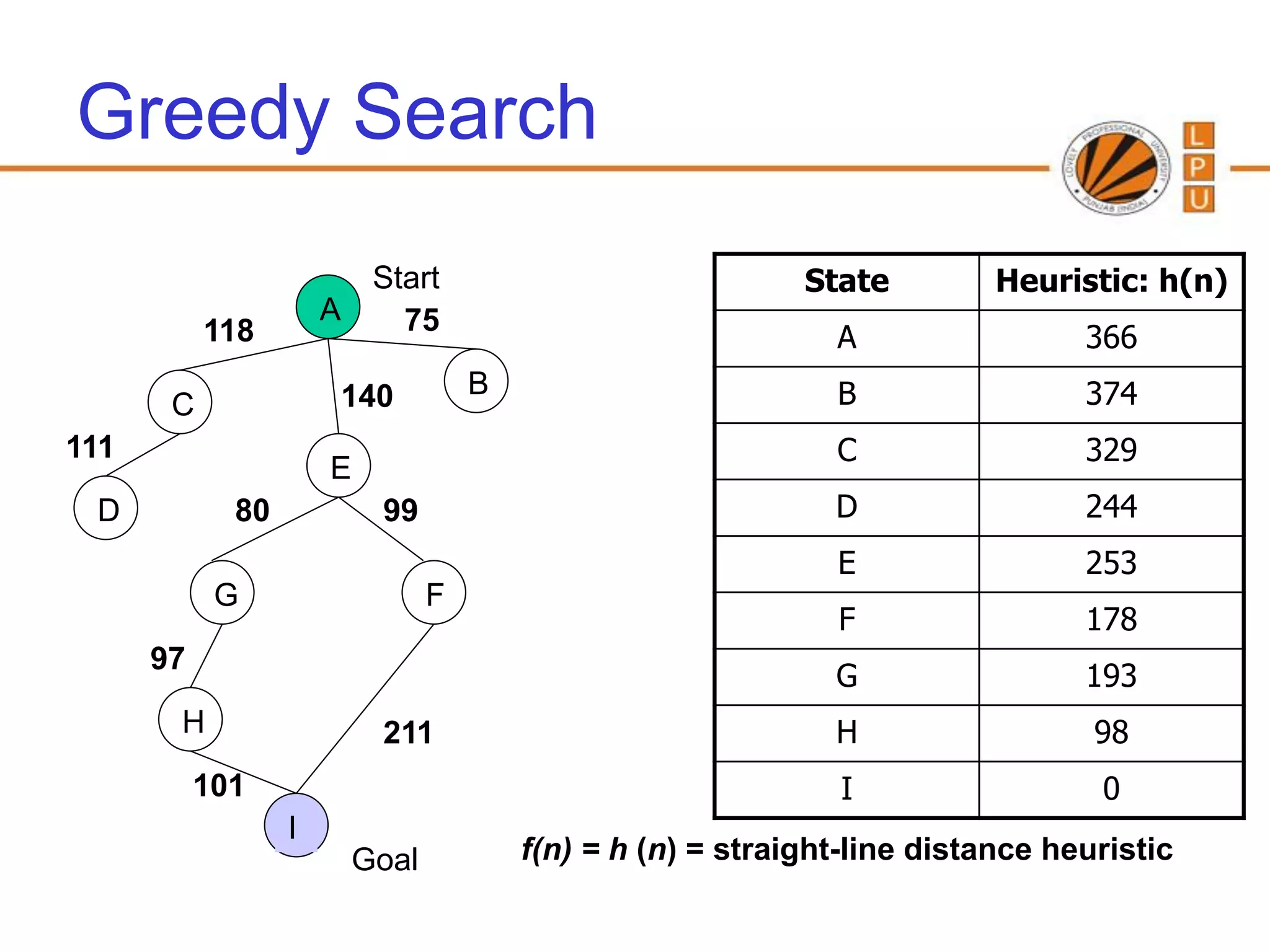
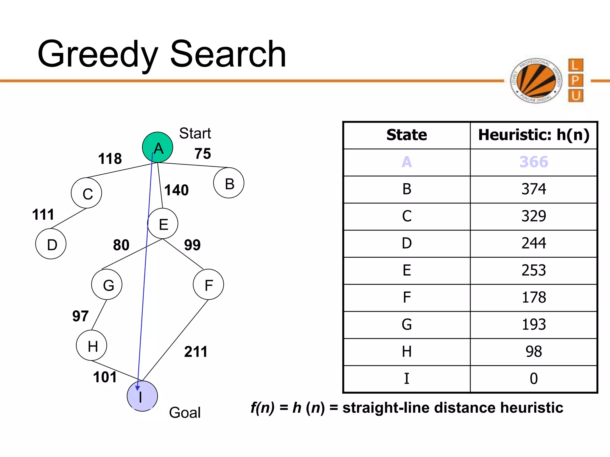
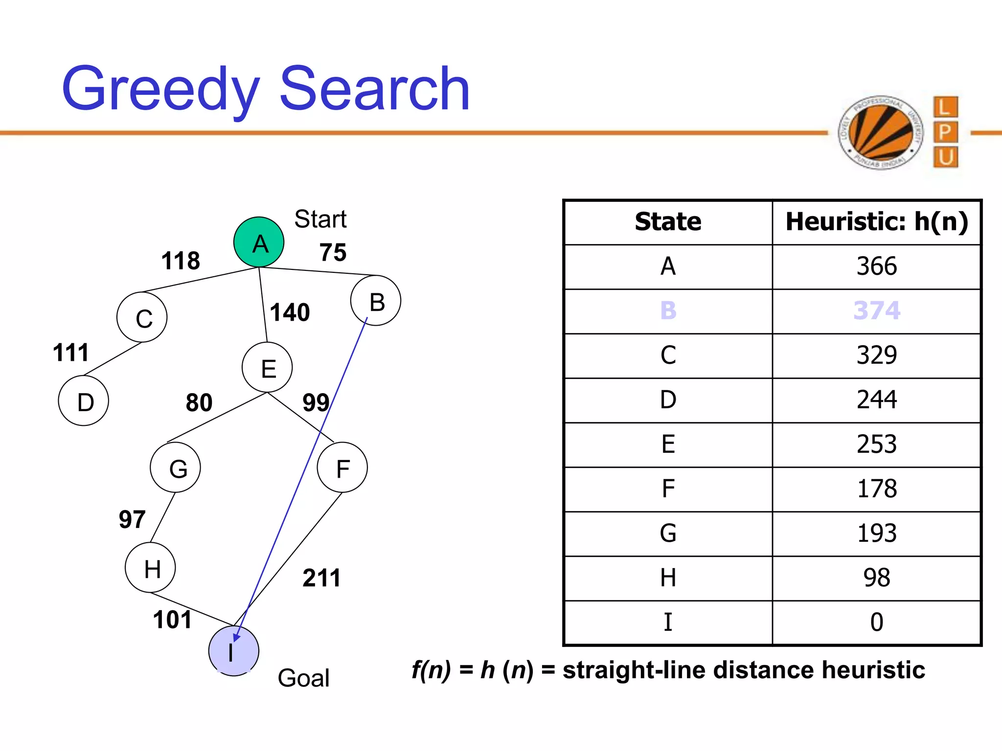
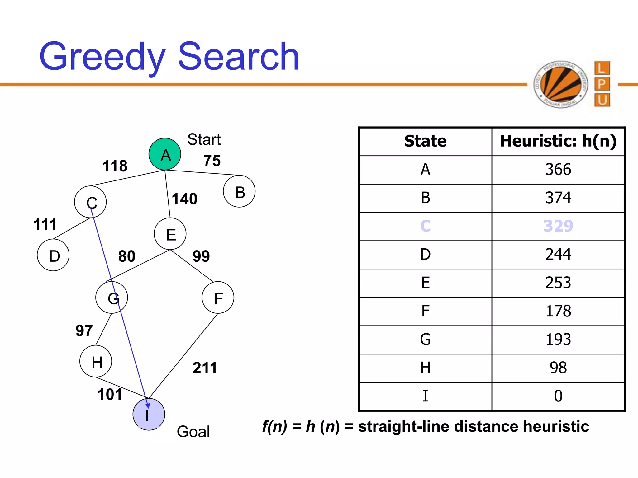
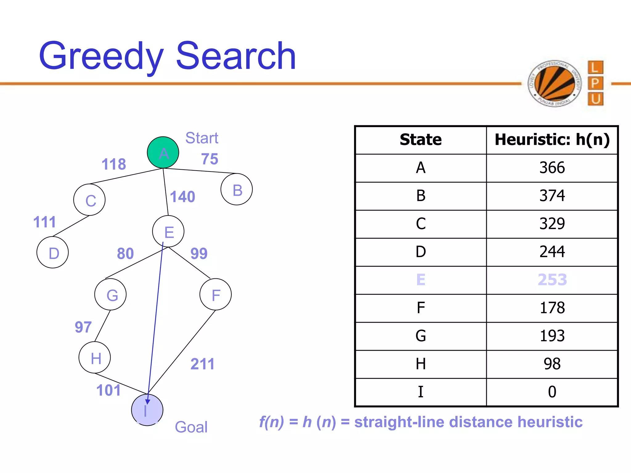
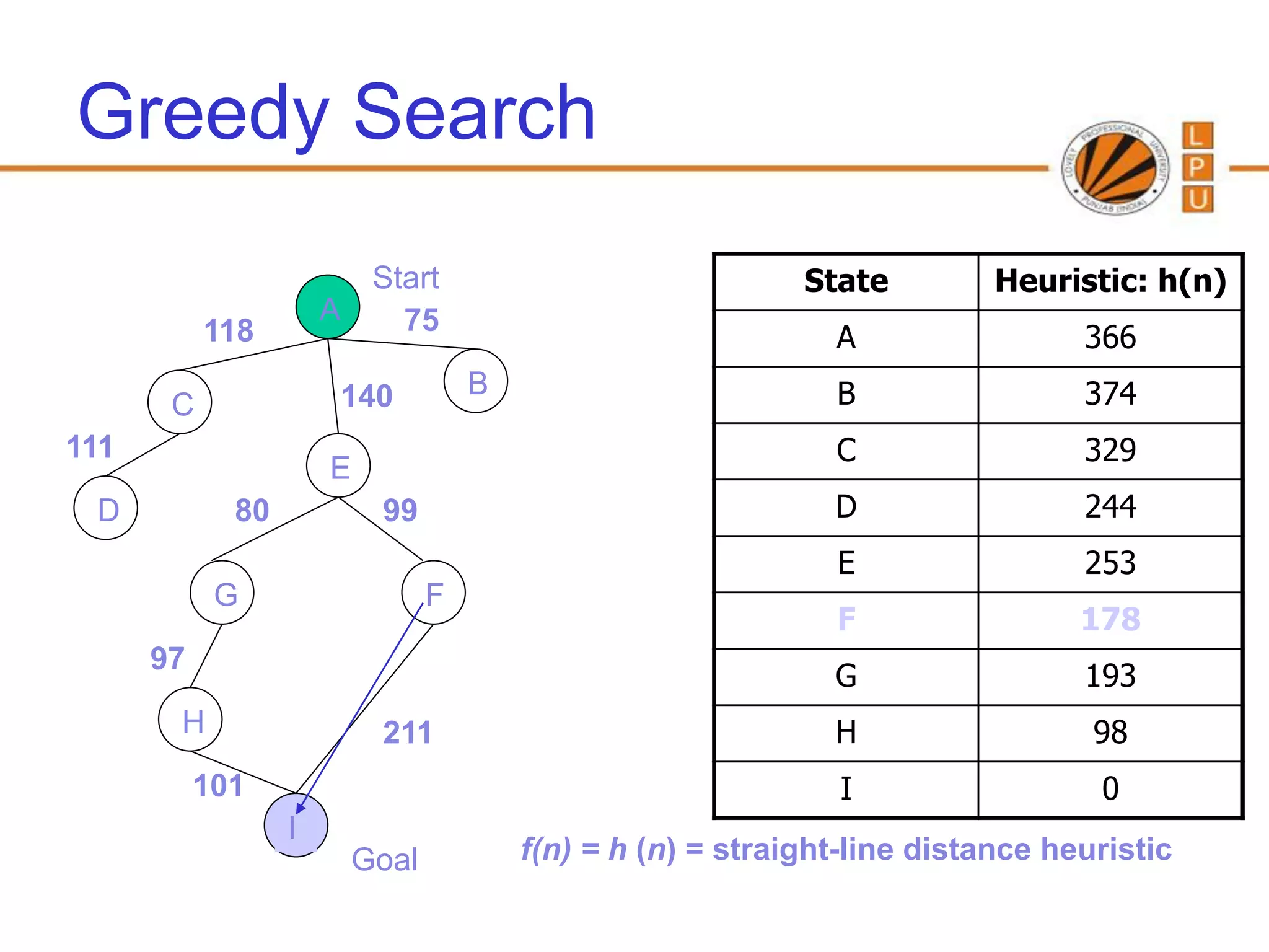
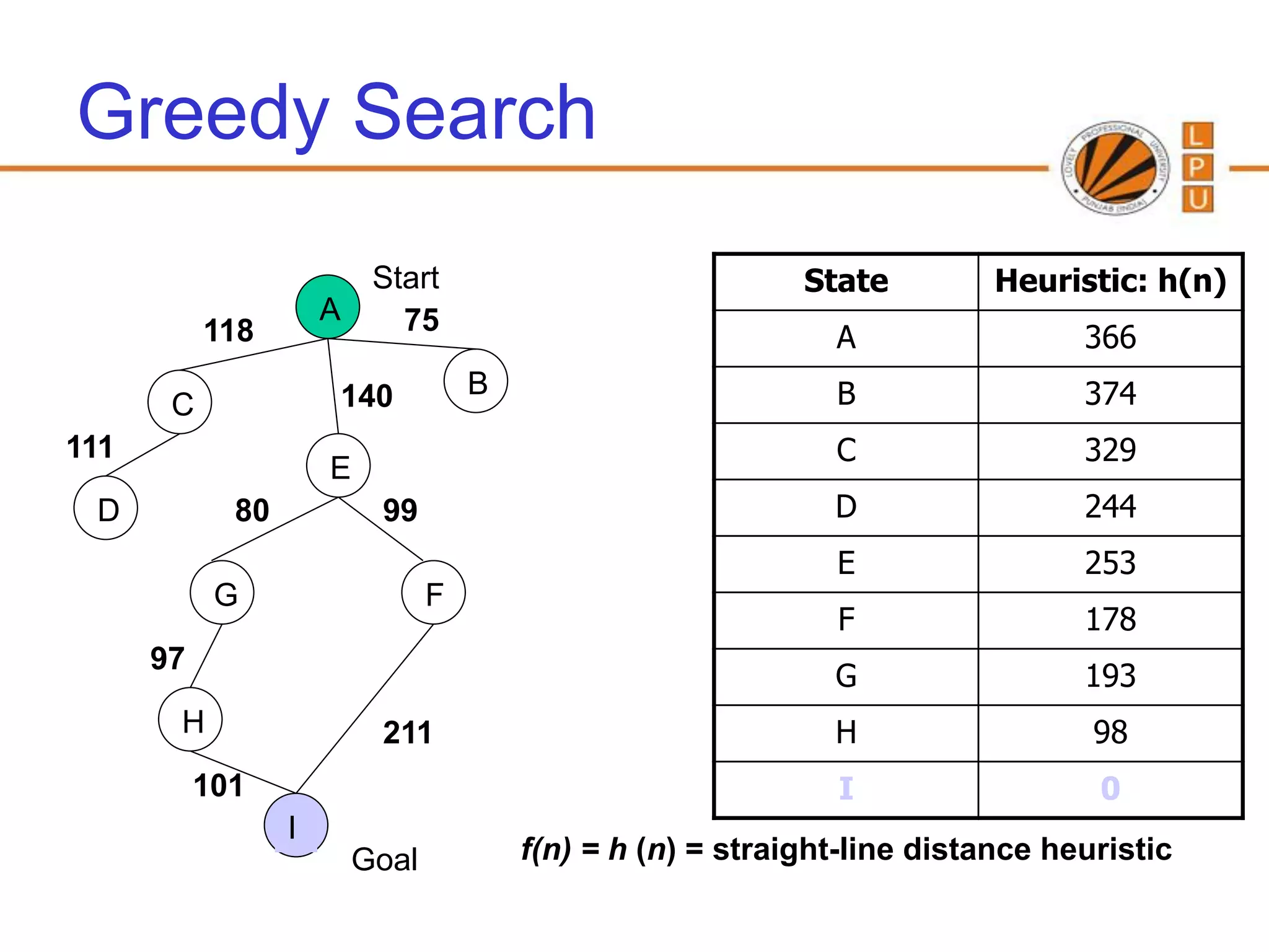
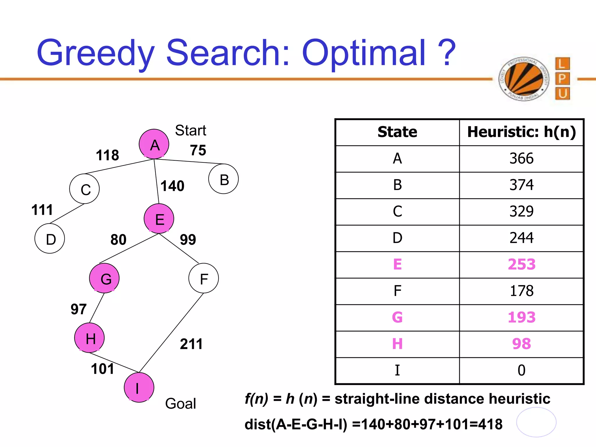
The document discusses heuristic search techniques for artificial intelligence. It covers greedy search which uses a heuristic function f(n) = h(n) to choose the successor node with the lowest estimated cost to reach the goal. An example of the travelling salesman problem is provided to illustrate greedy search.
Overview of AI concepts, problem-solving techniques including state-space search, control strategies, and exhaustive search methods.
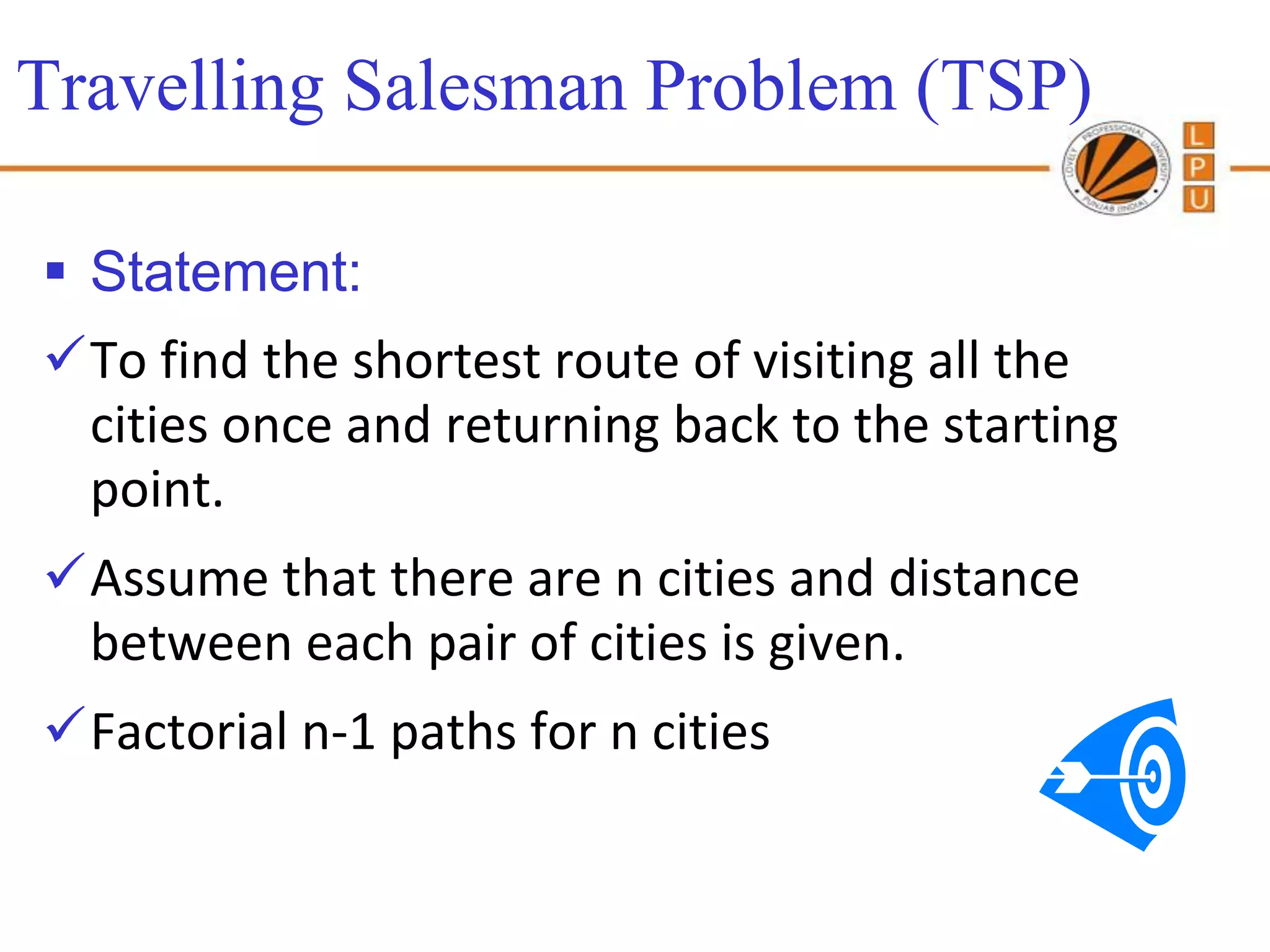
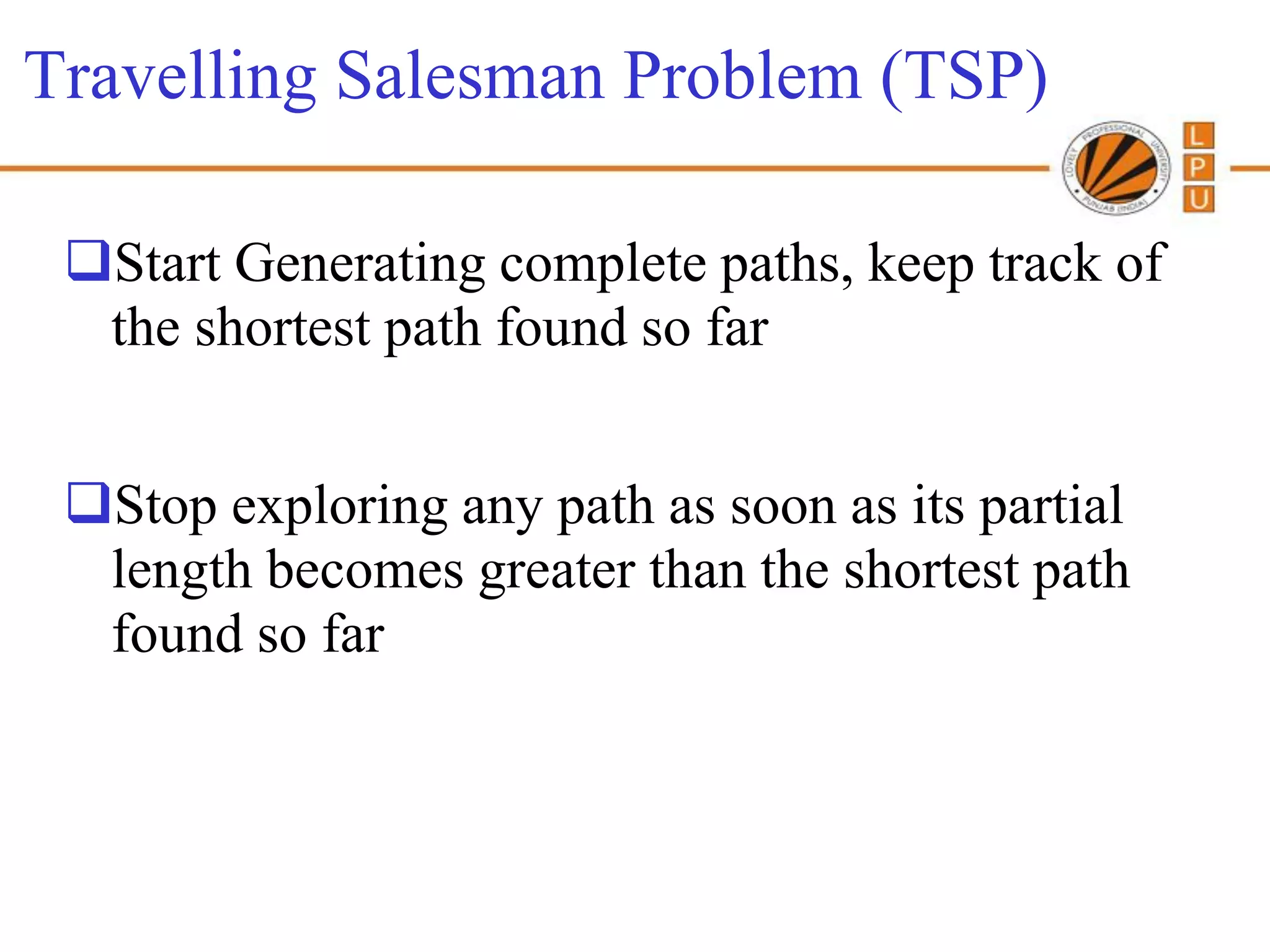
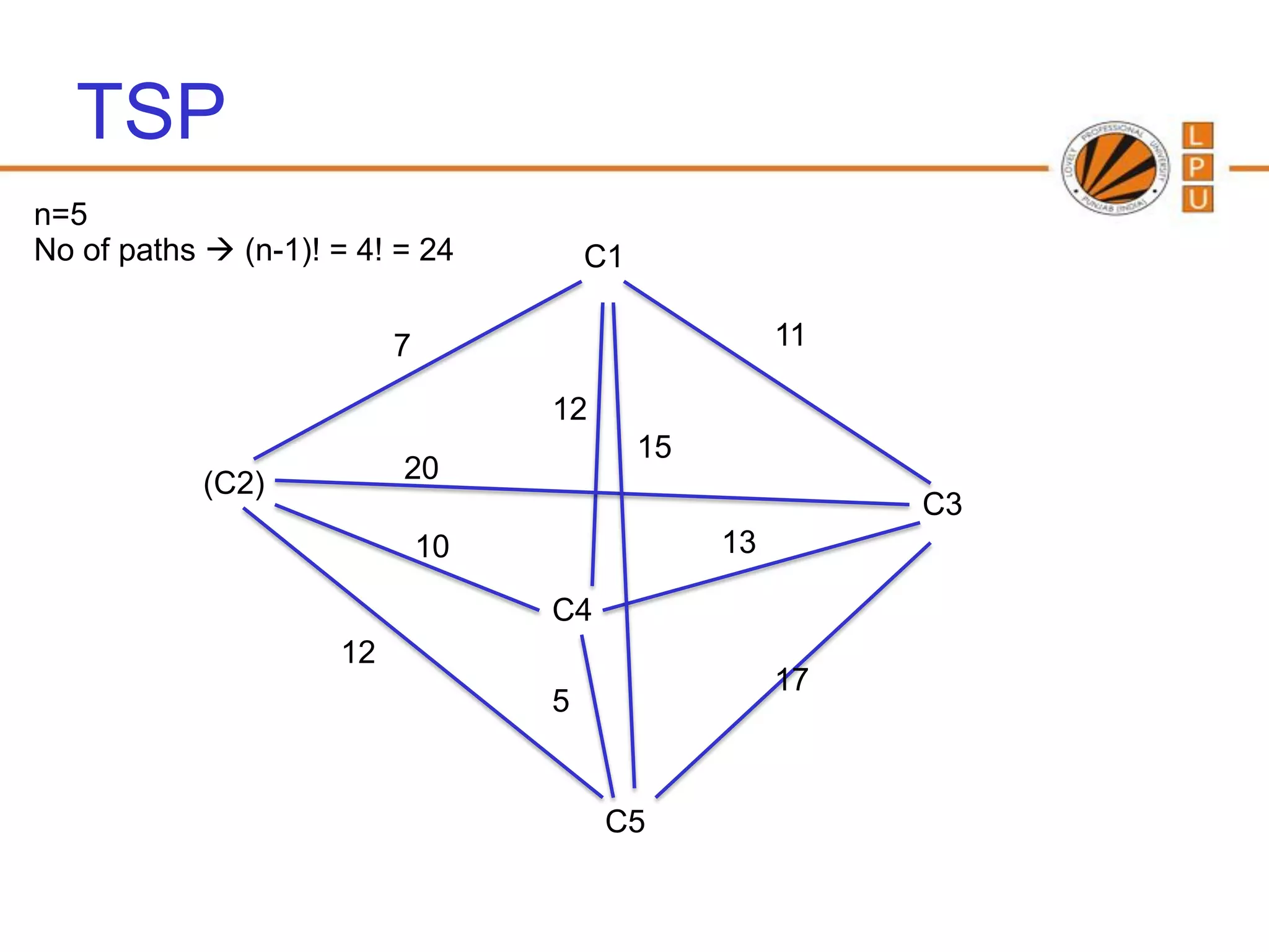
Discussion on TSP, aiming to find the shortest route visiting n cities with factorial paths.
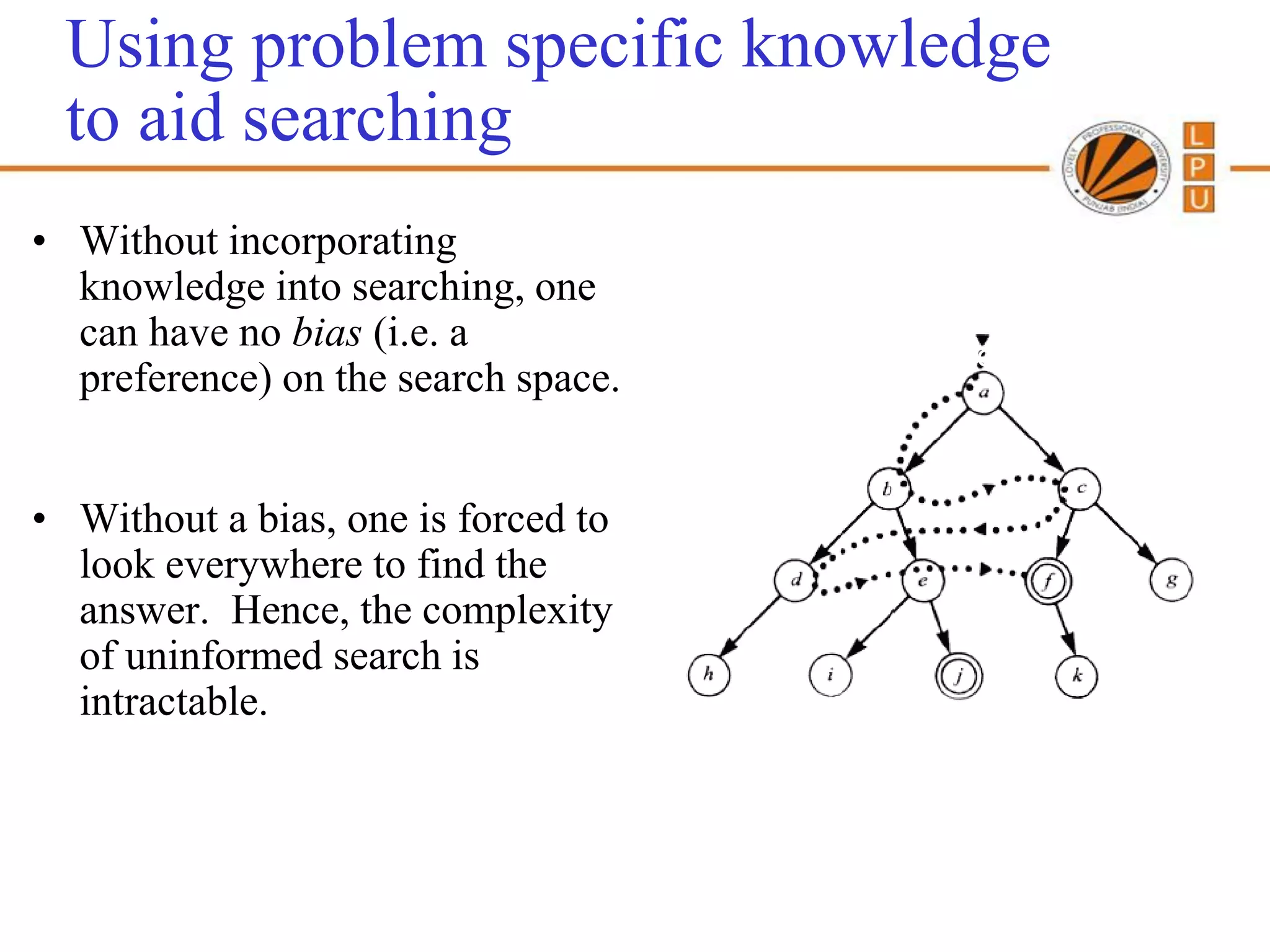
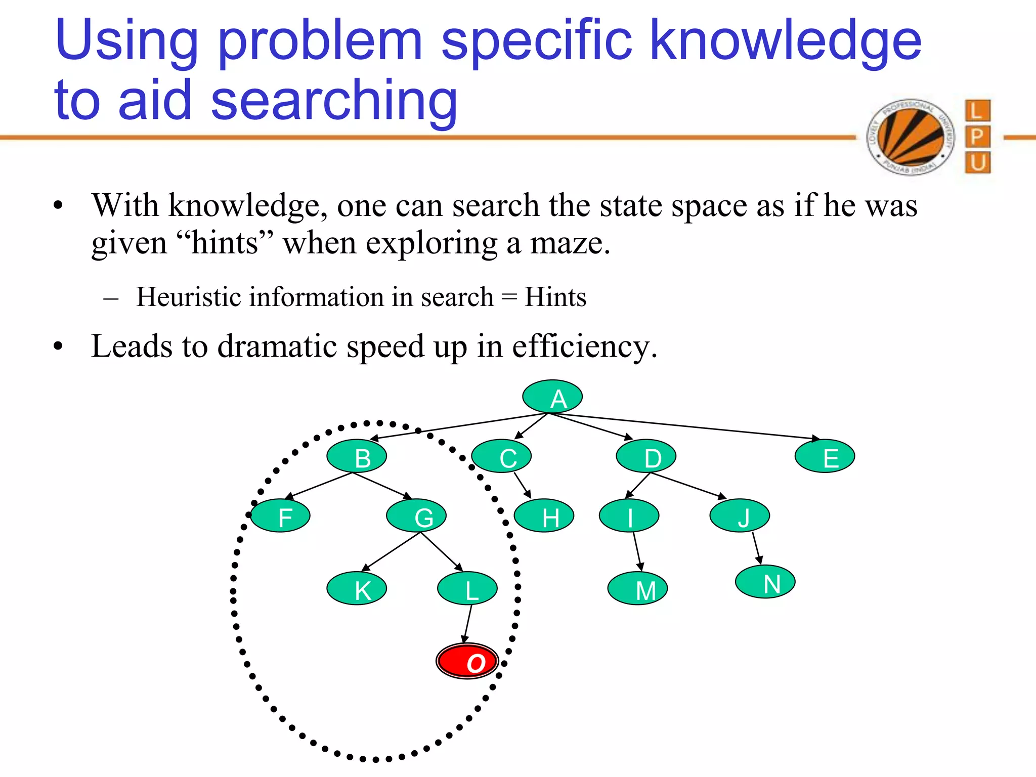
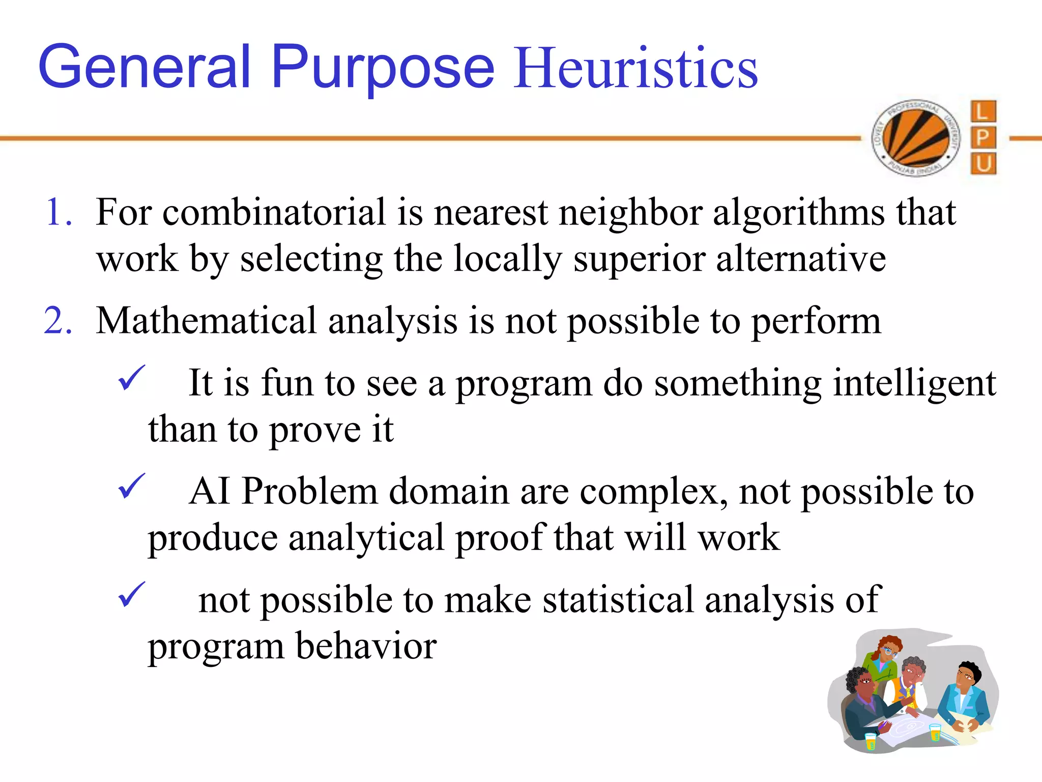
Use of problem-specific knowledge in searching to avoid exhaustive methods; introduction to general and special purpose heuristics.
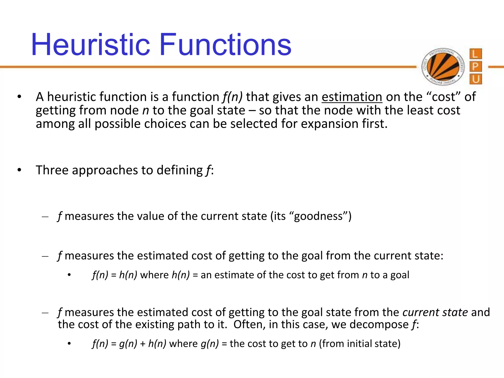
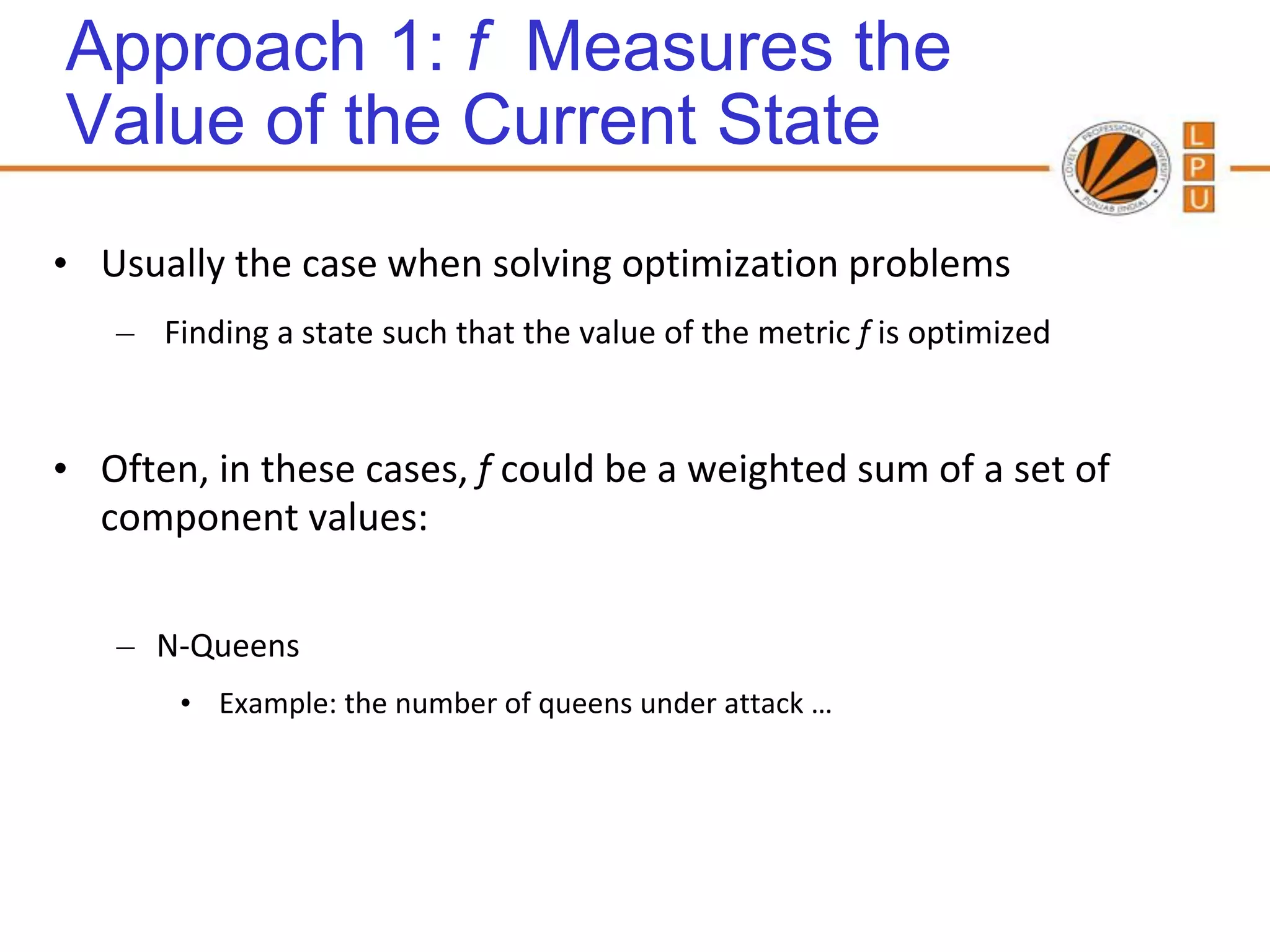
Explanation of heuristic functions that estimate costs; methods to define heuristics (f-values).
Introduction to informed search strategies like Greedy Best First and A* algorithms.
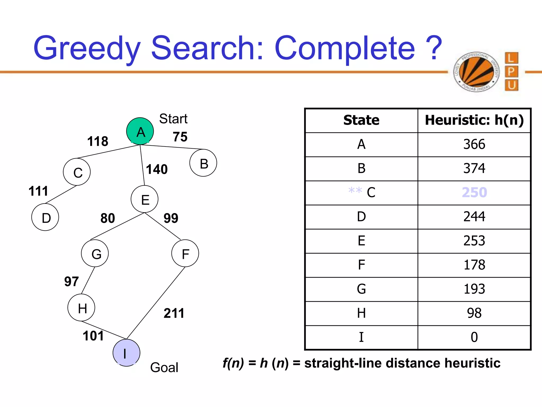
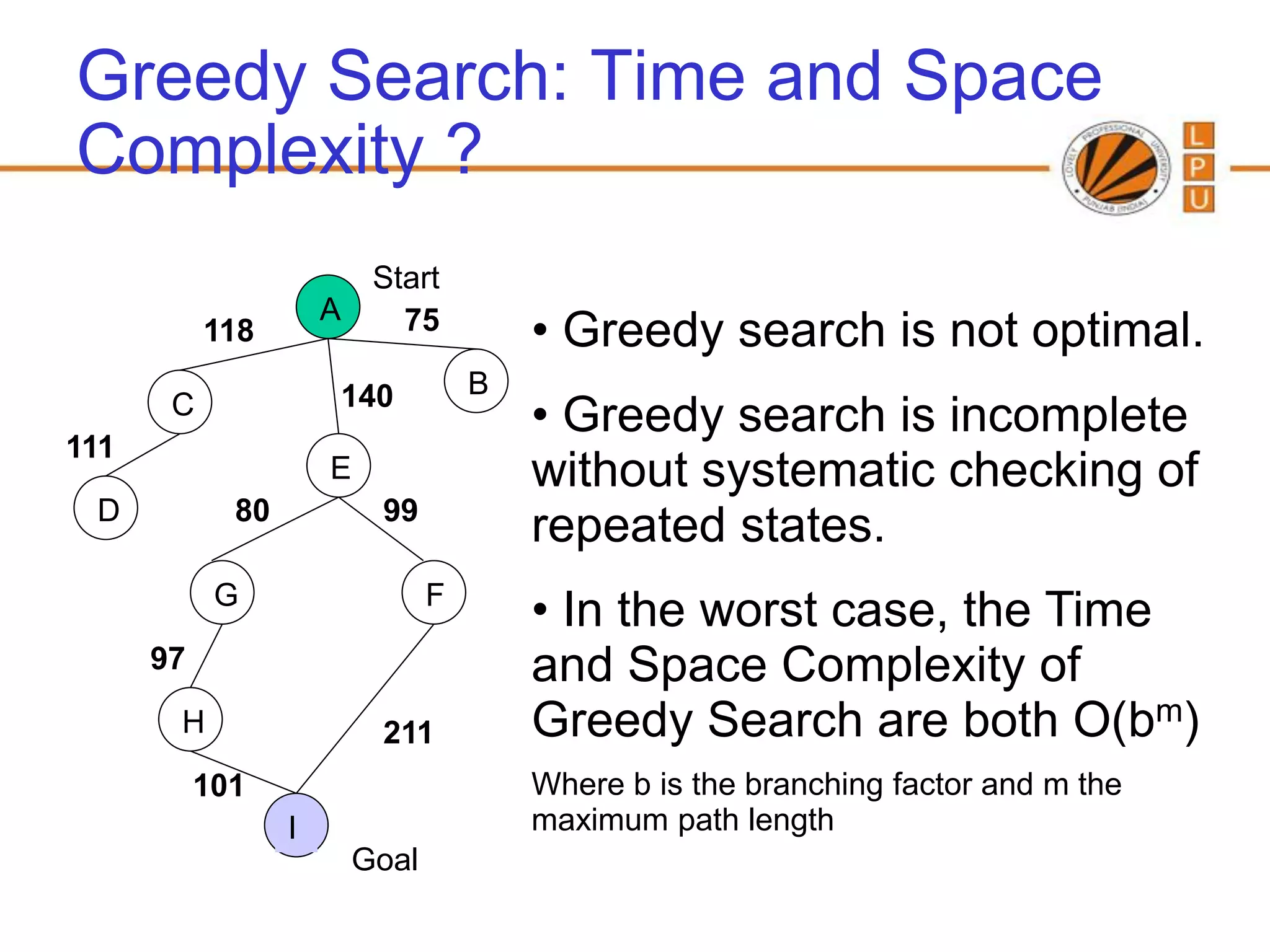
Detailed explanation of Greedy Search, using examples and the concept of heuristic functions.
Explaining UCS, its optimality under equal costs, and its handling of path costs for efficient searches.
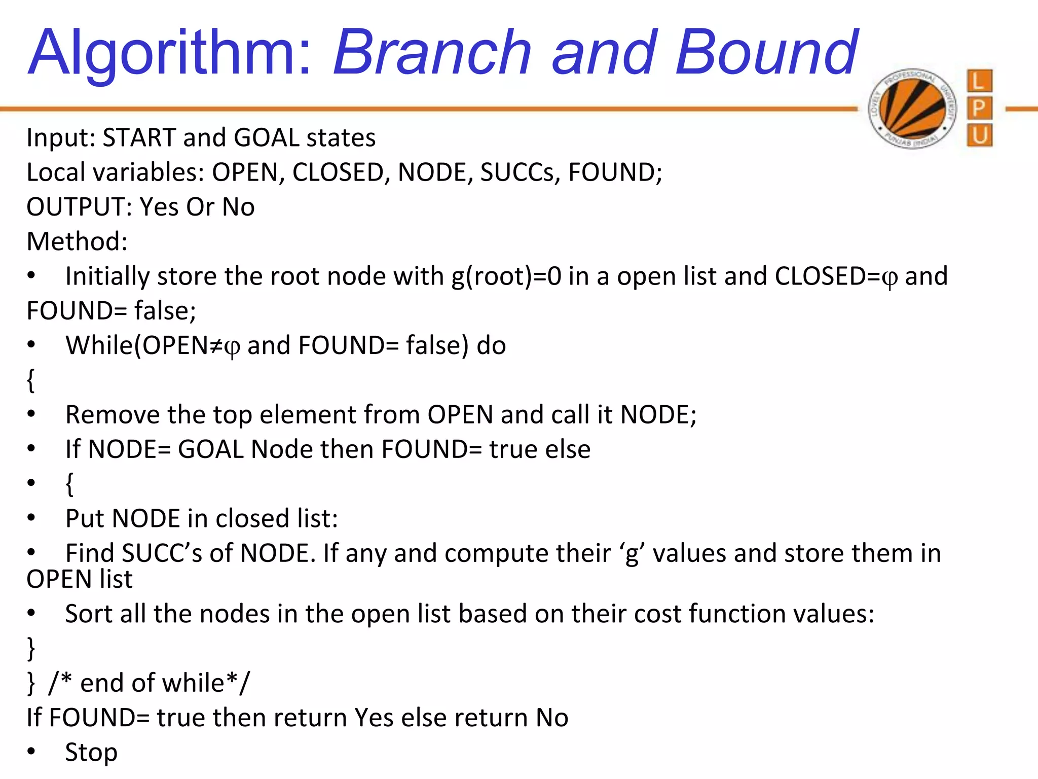
Description of branch and bound algorithms in searching for optimal paths.
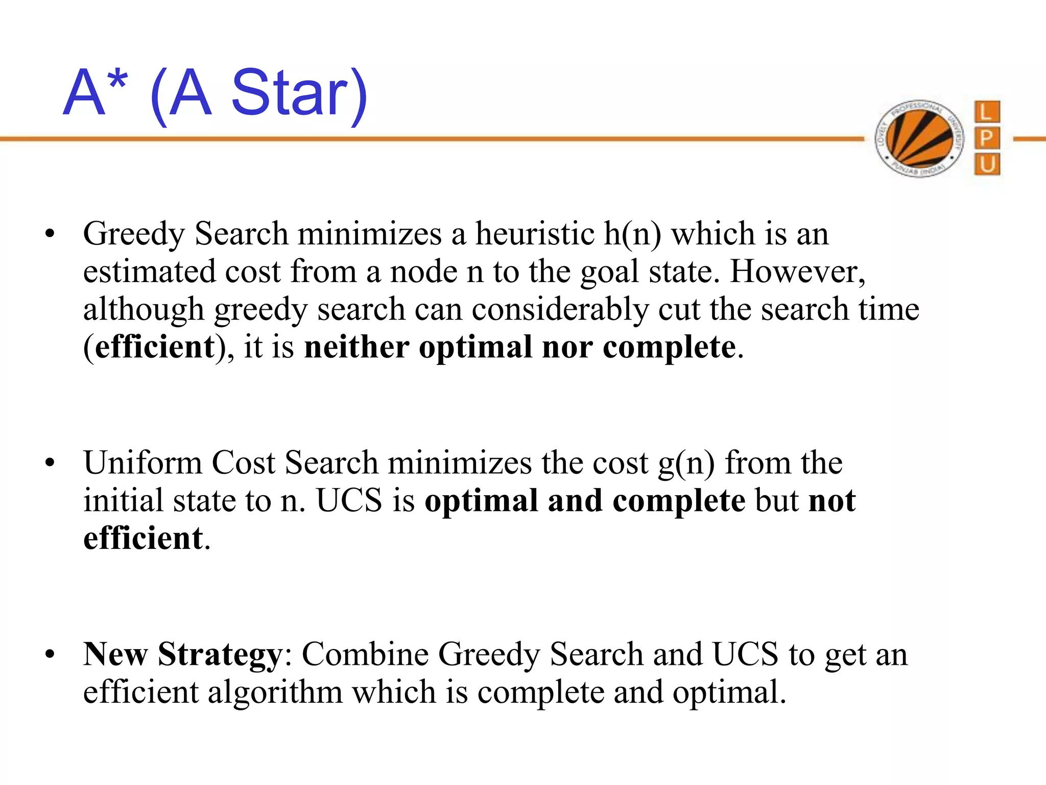
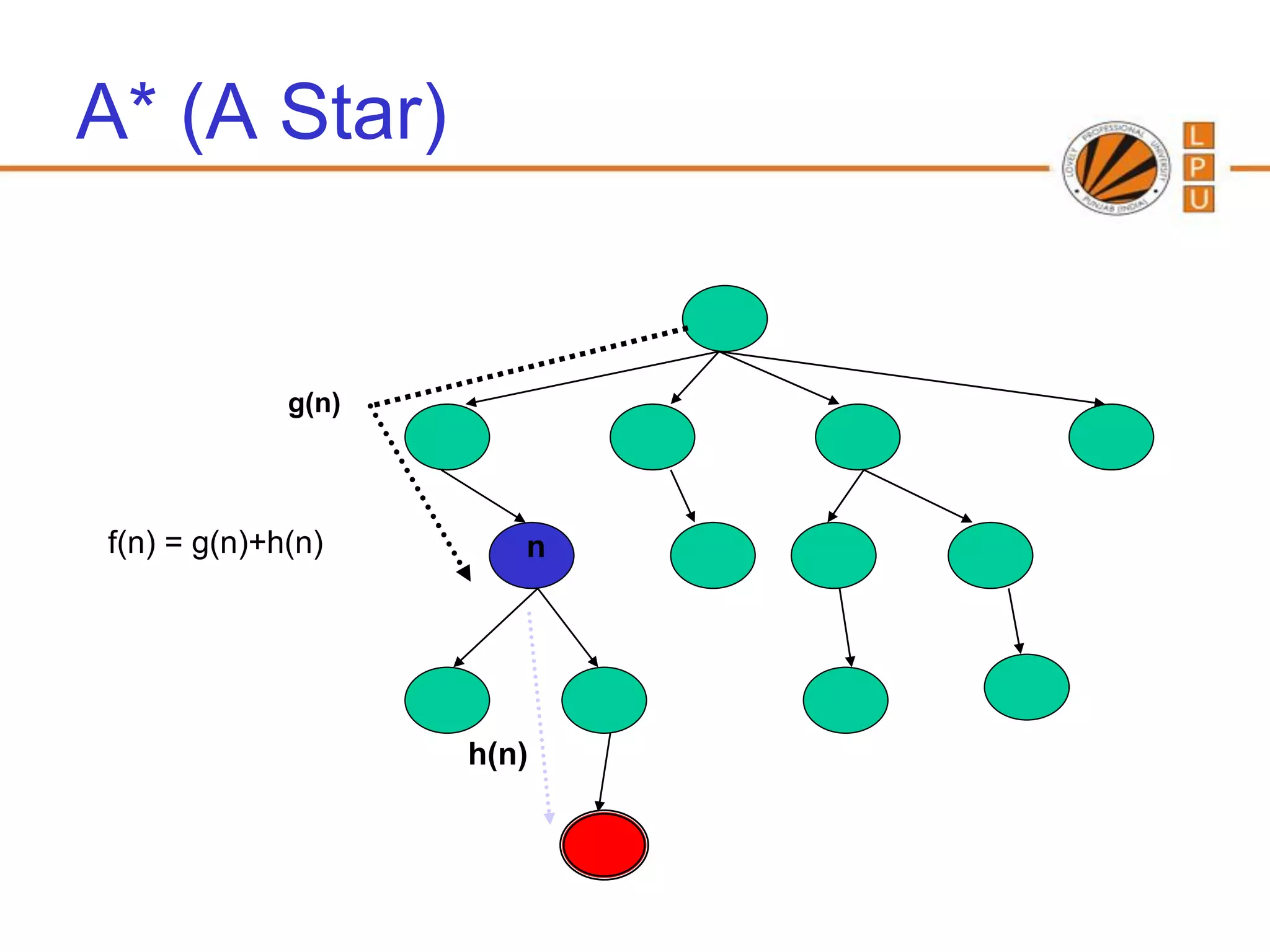
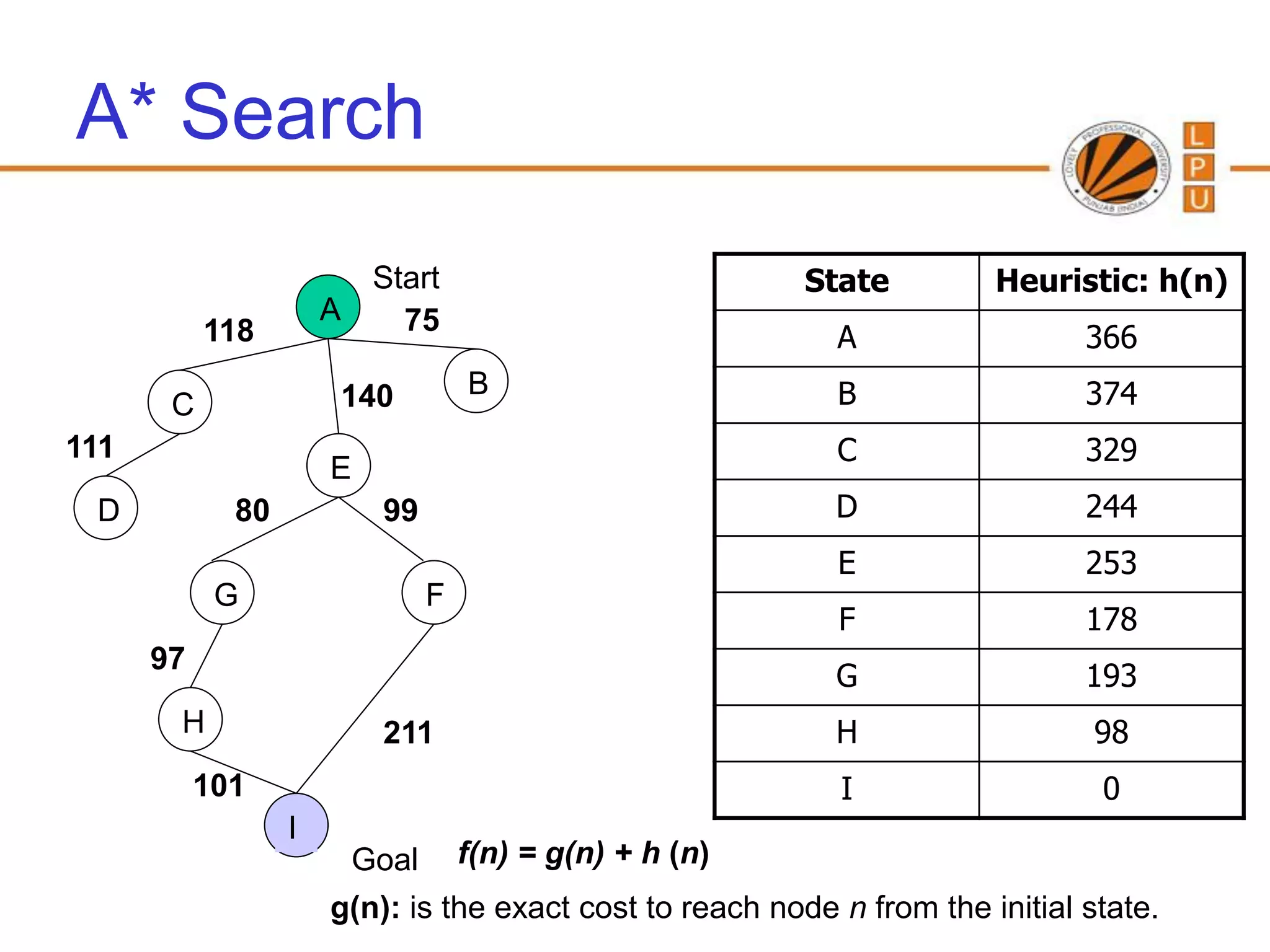
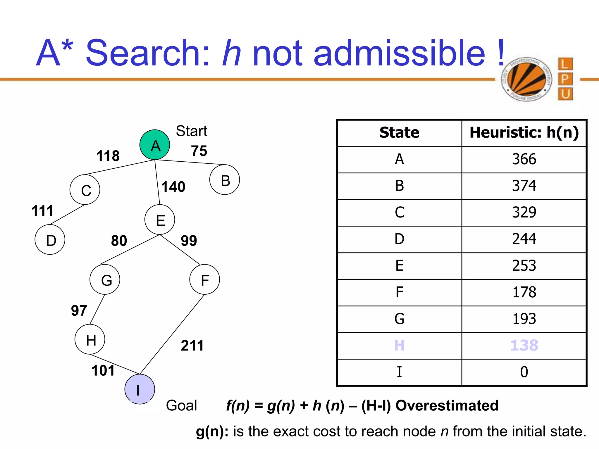
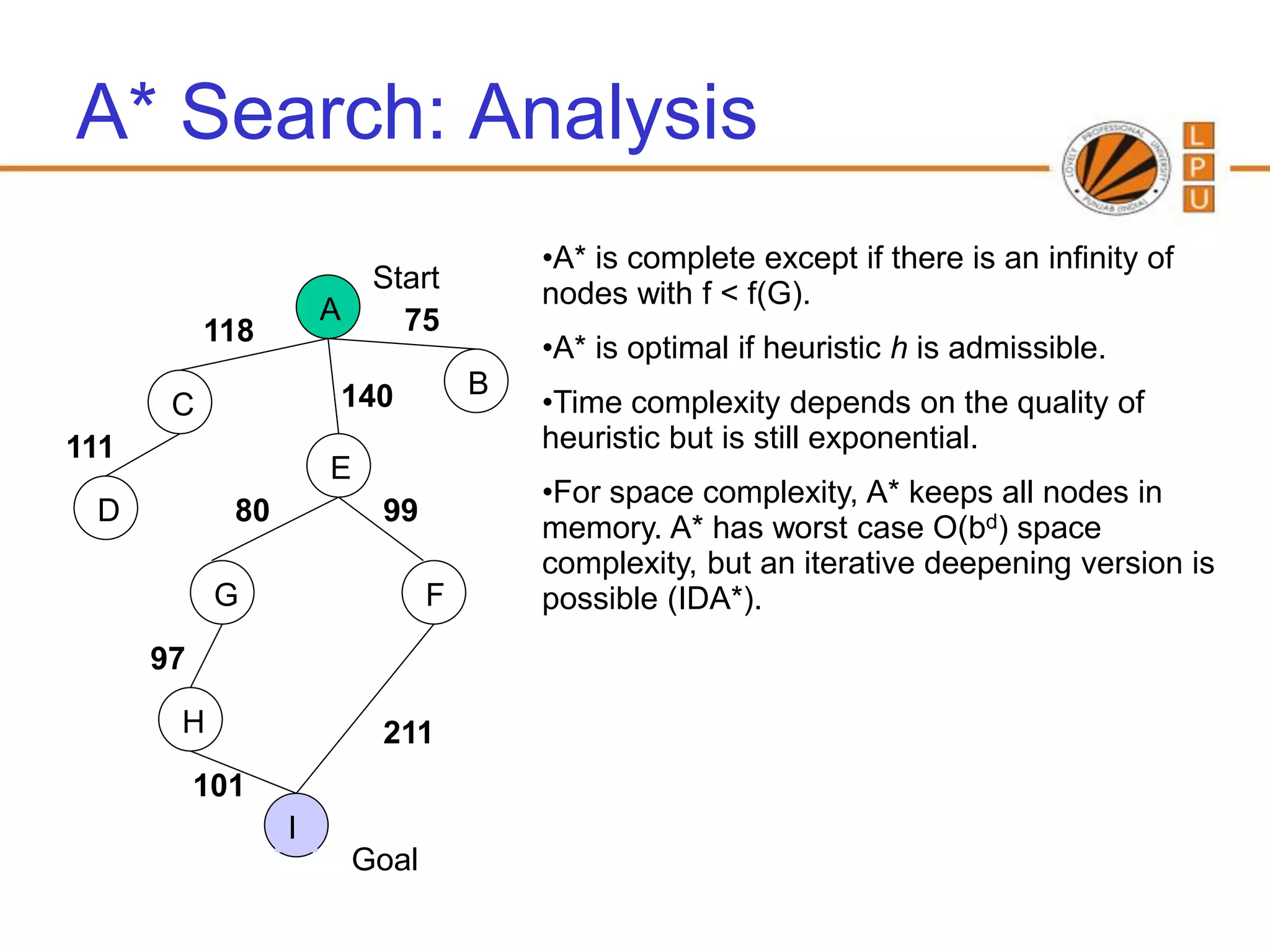
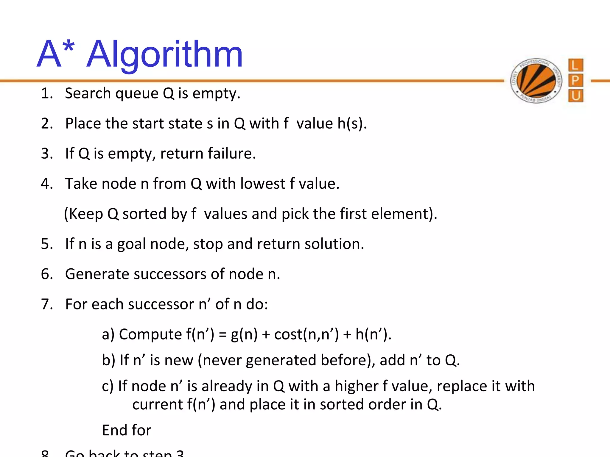
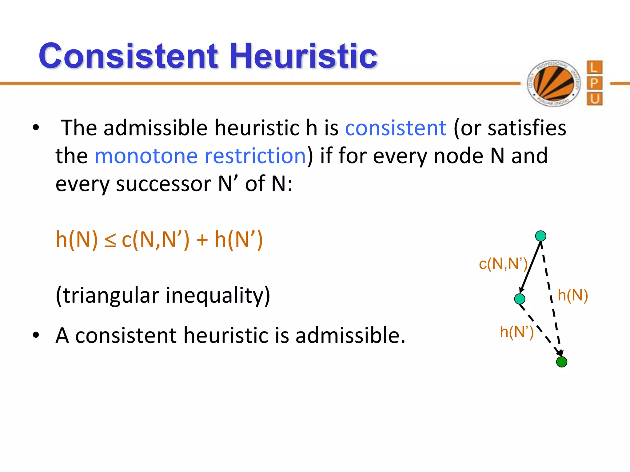
A comprehensive breakdown of the A* search method, combining heuristic and cost functions for optimal search paths.
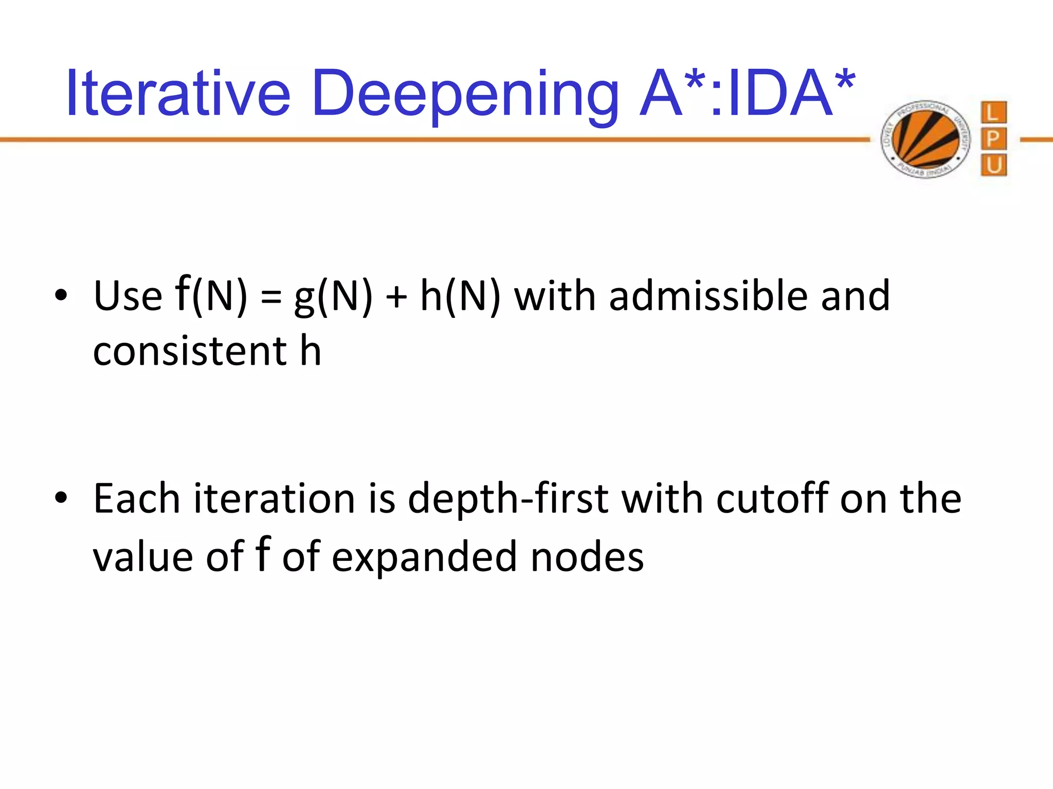
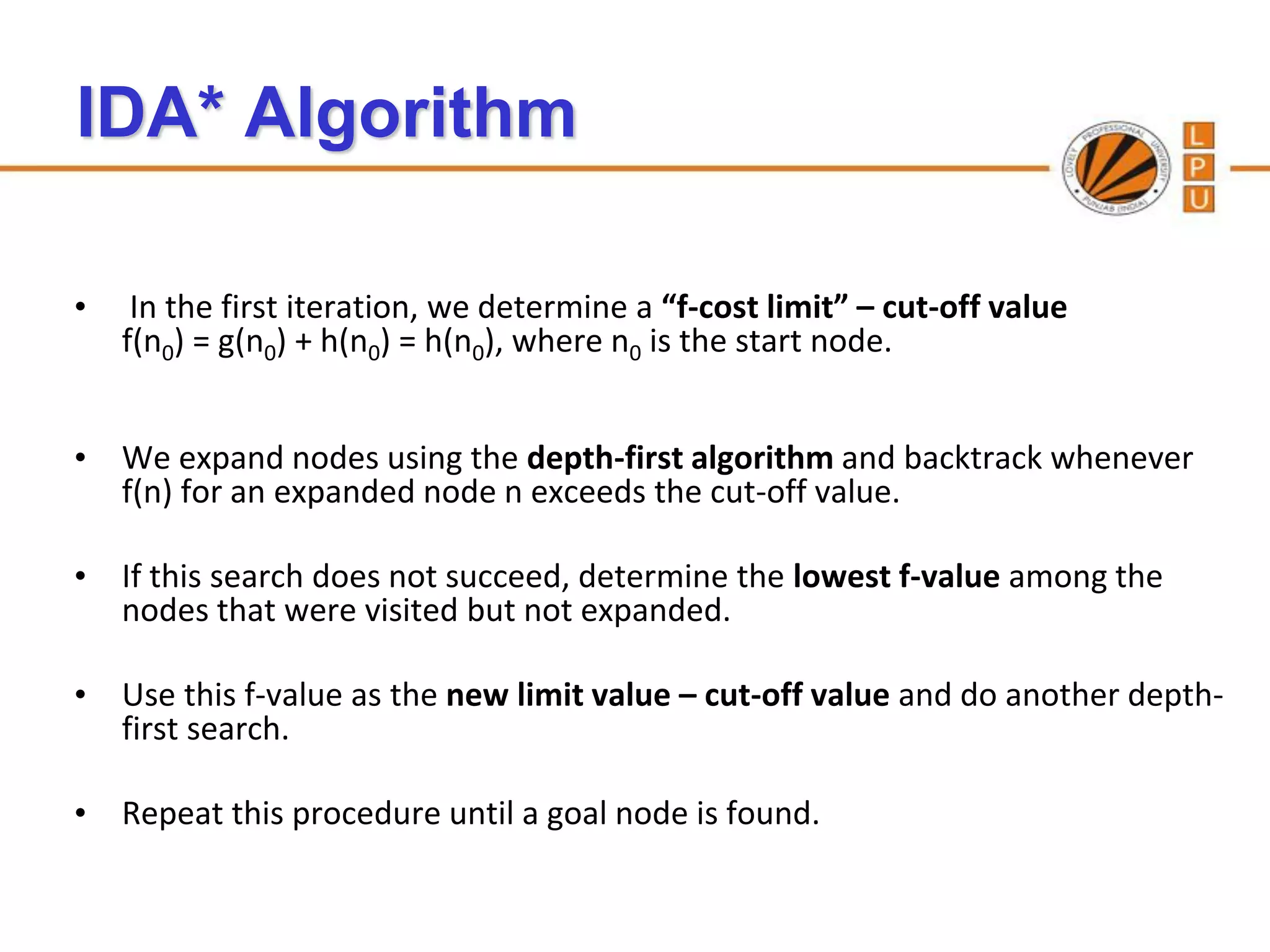
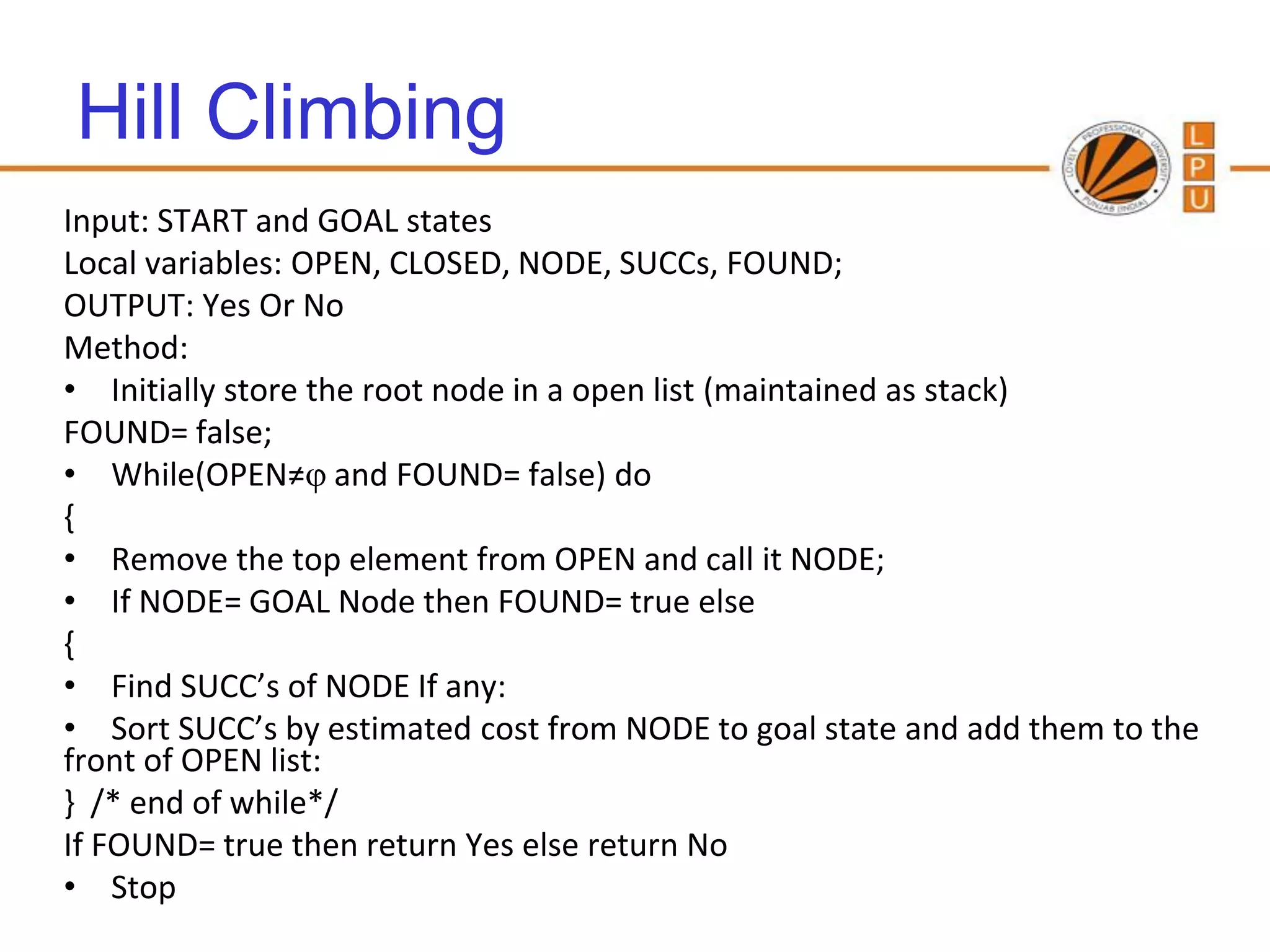
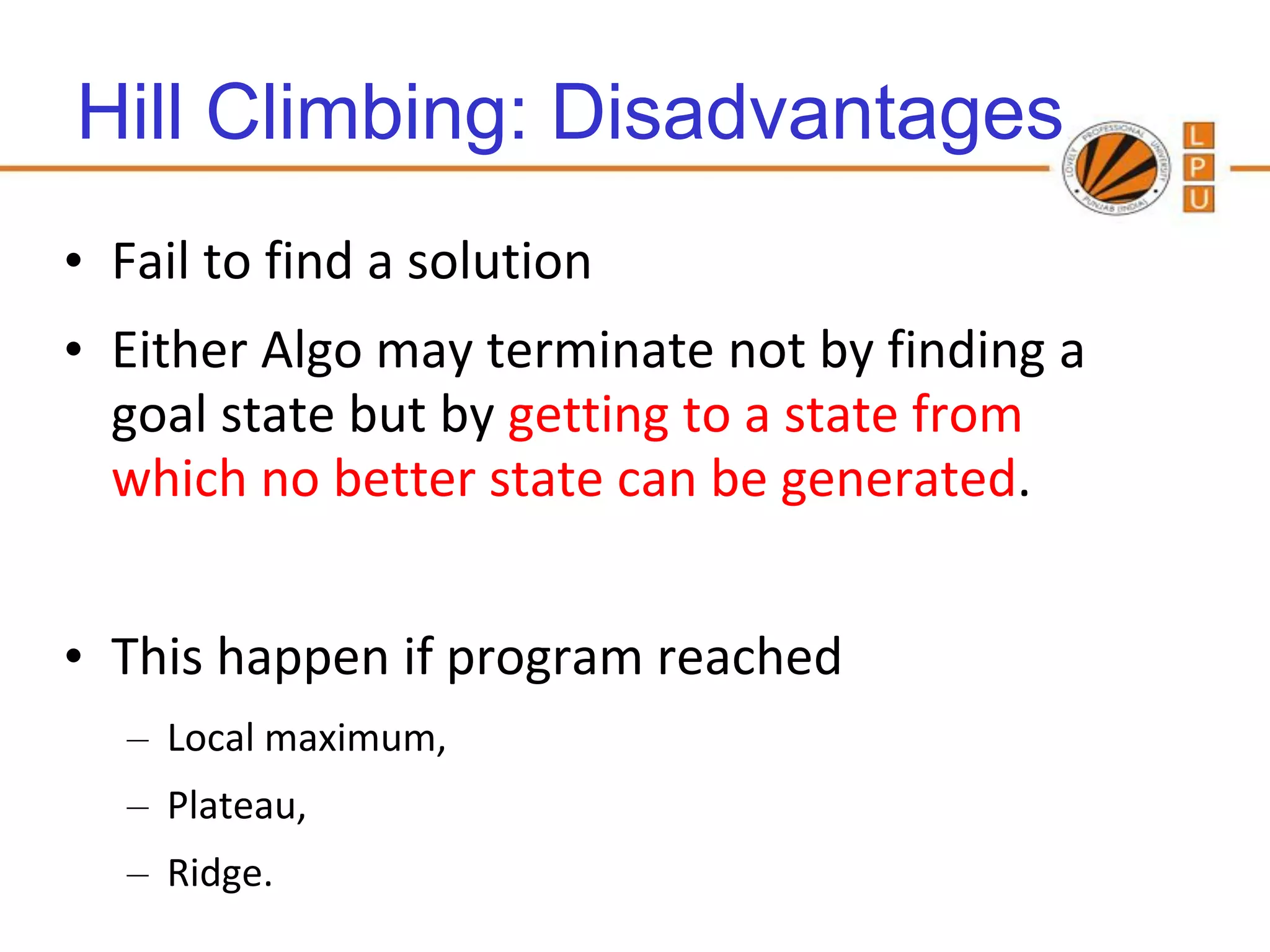
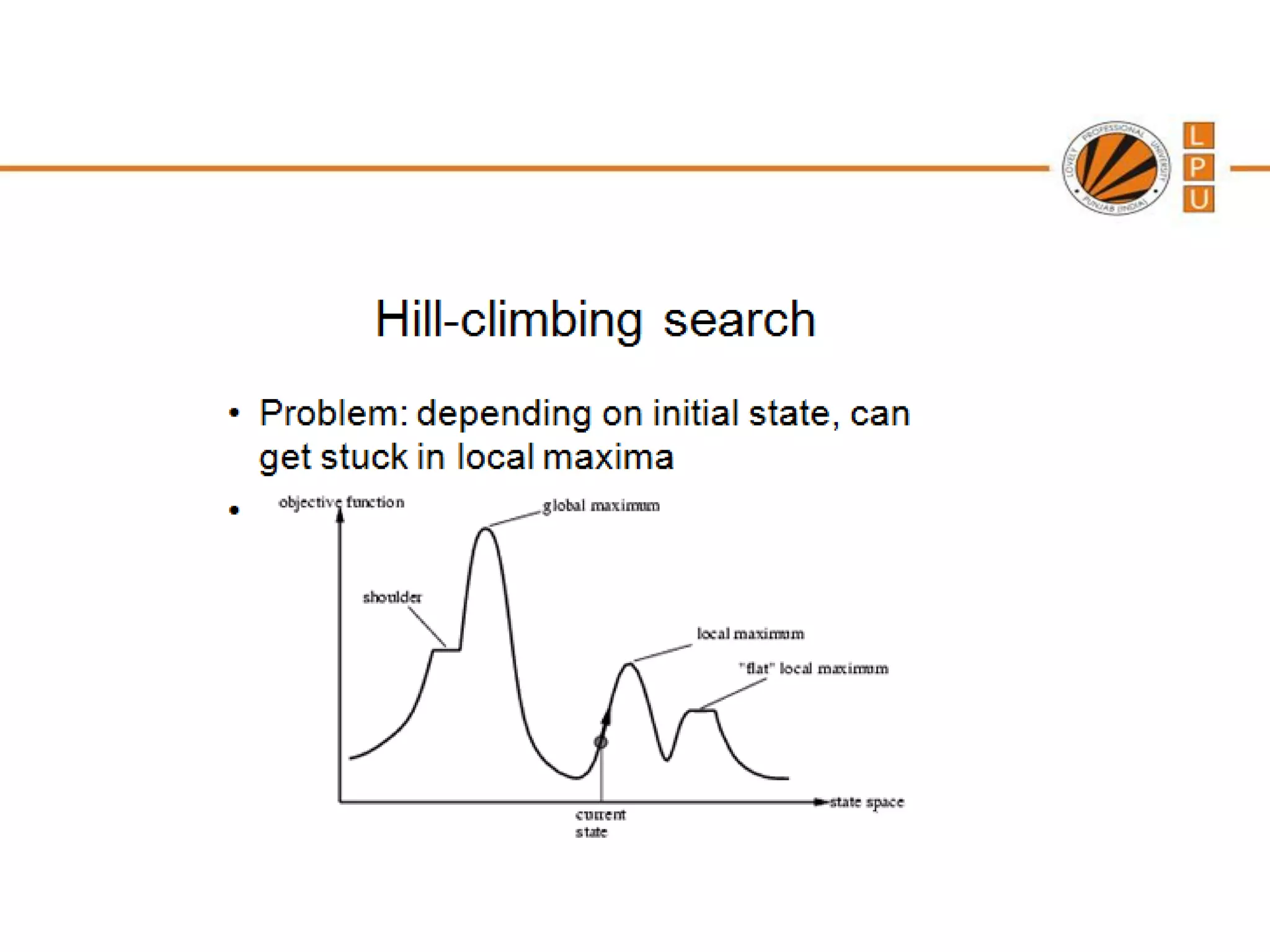
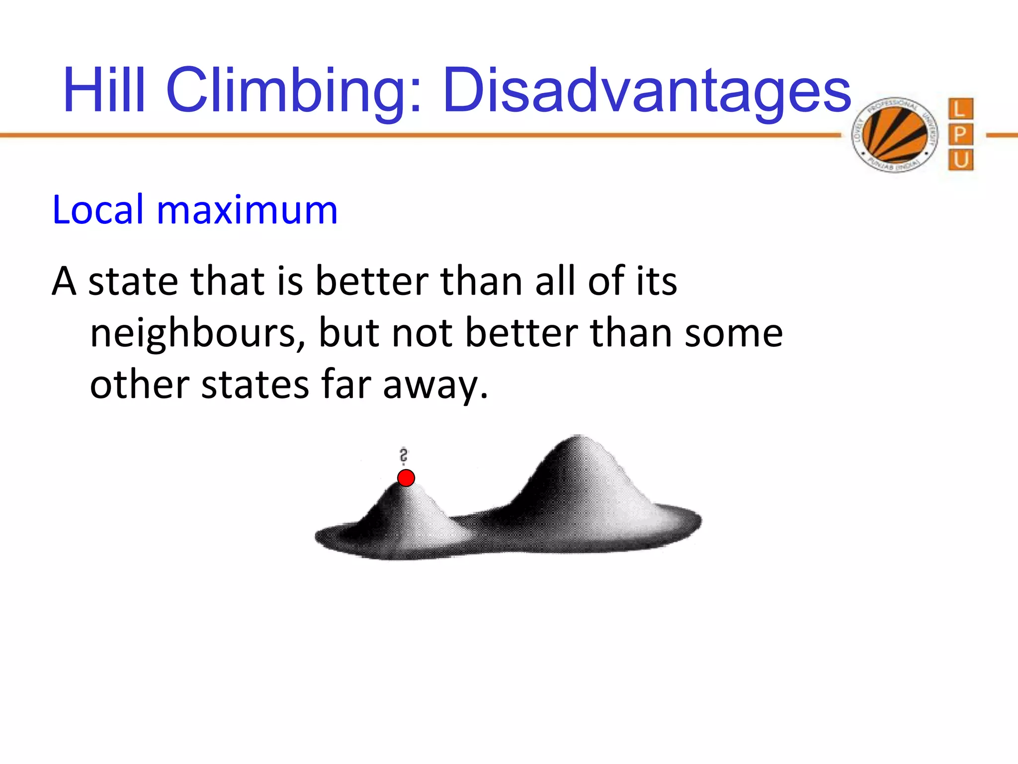
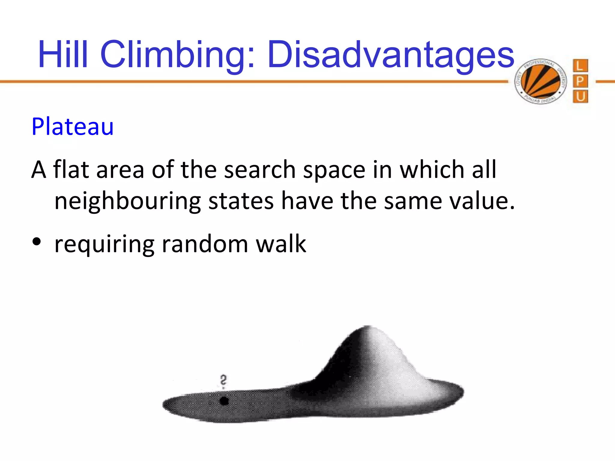
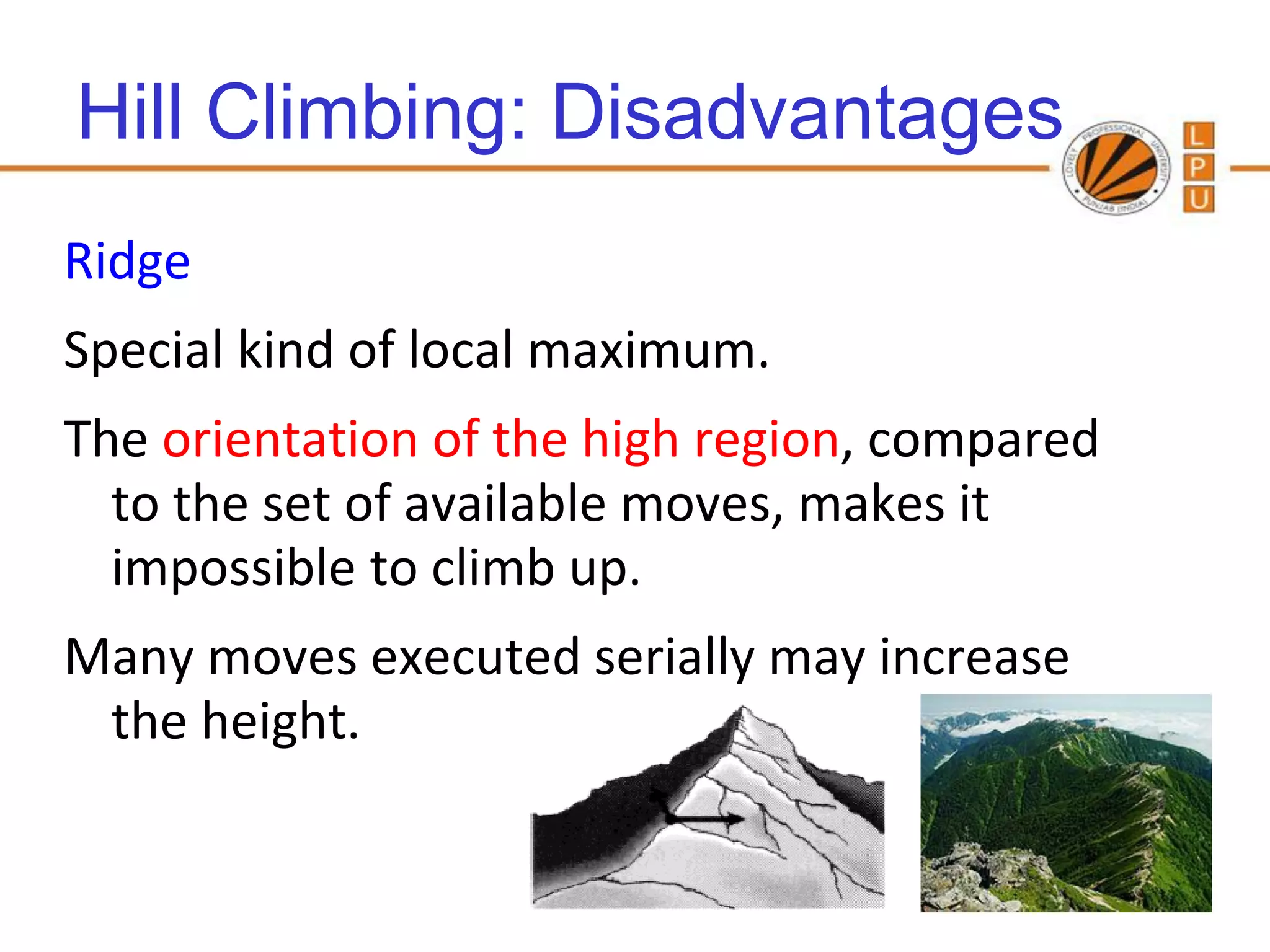
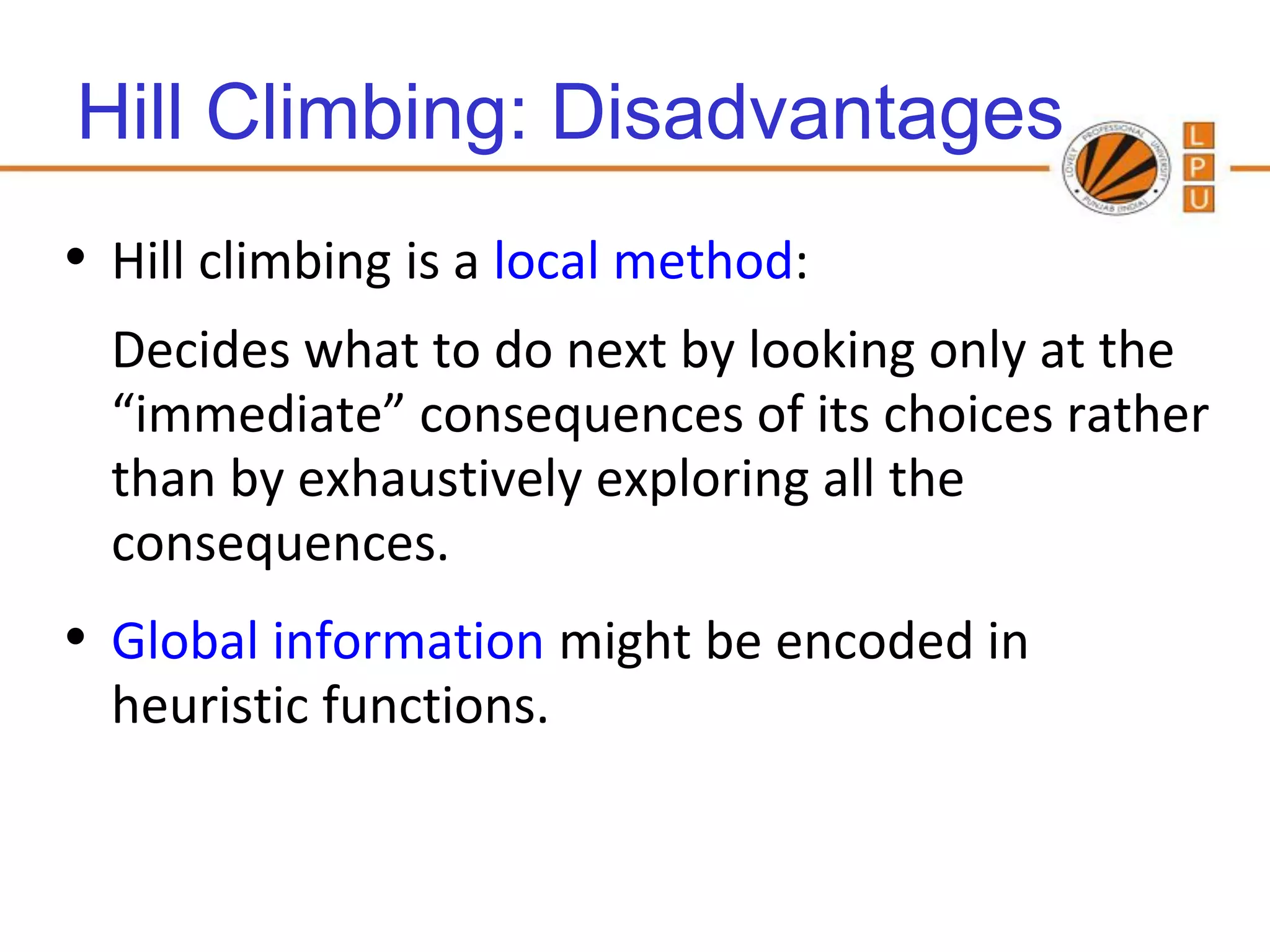
Introduction to Iterative Deepening A*, Hill Climbing methods, their advantages, and limitations.
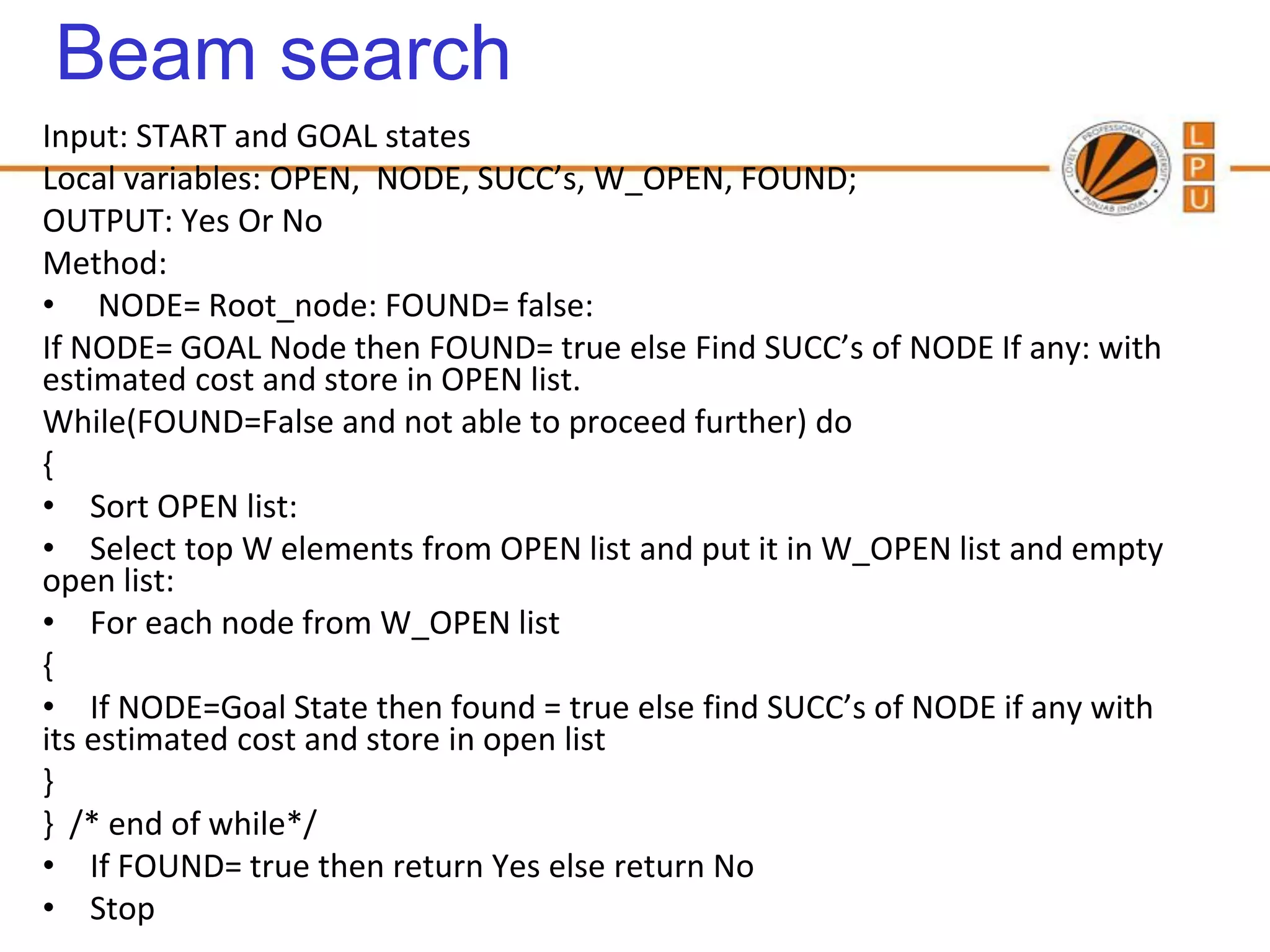
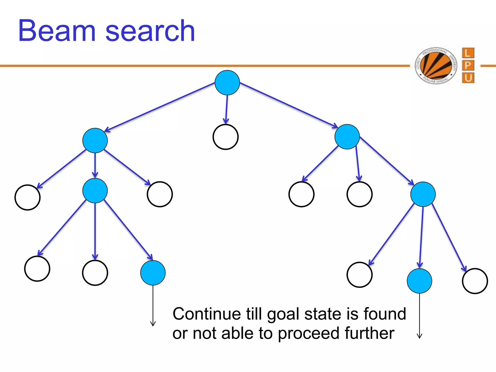
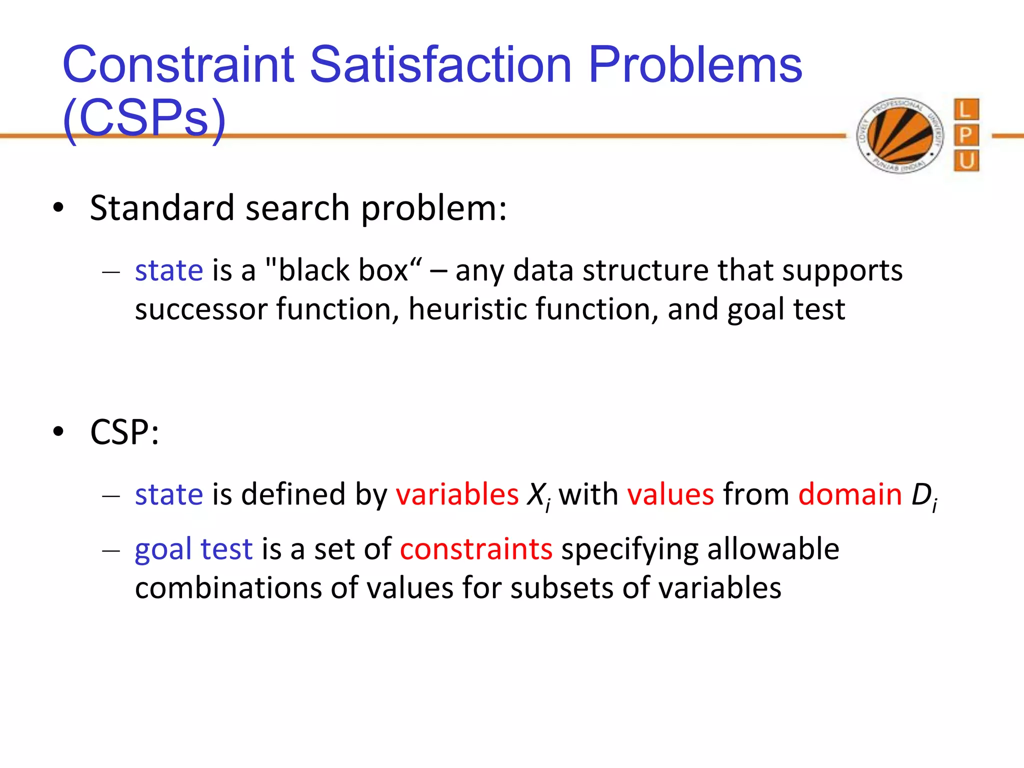
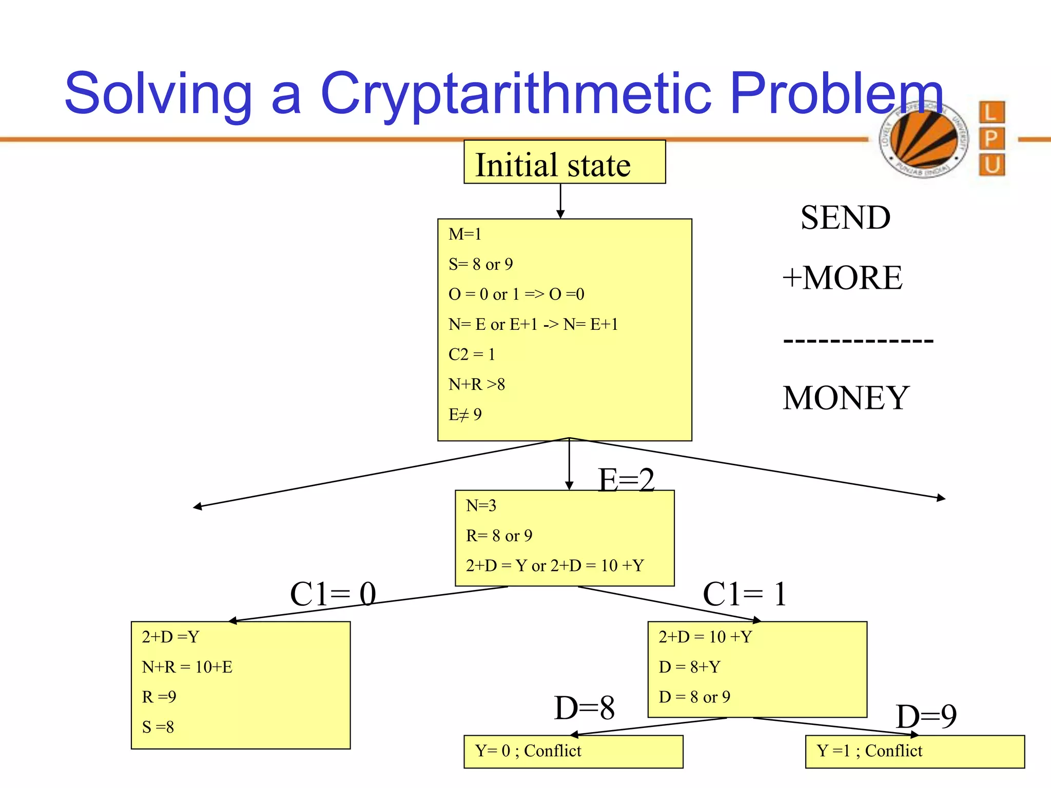
Description of Beam Search and Constraint Satisfaction Problems in AI, with examples and solution strategies.
Summary of insights on informed heuristic search strategies and their importance in enhancing search efficiency.


![Heuristic in AI (Rule of thumb) [what, why, how] What: Mental shortcuts that ...](https://cdn.slidesharecdn.com/ss_thumbnails/3-5-week-250901055018-f7c36e71-thumbnail.jpg?width=640&height=640&fit=bounds)


