UPDATED UNIT 4 DBMS NOTES ECE DS SRM 21 Reg

Transaction Concept
• A transaction is a unit of program execution that
accesses and possibly updates various data items.
• E.g., transaction to transfer $50 from account A to
account B:
1. read(A)
2. A := A – 50
3. write(A)
4. read(B)
5. B := B + 50
6. write(B)
• Two main issues to deal with:
• Failures of various kinds, such as hardware failures and
system crashes
• Concurrent execution of multiple transactions

ACID Properties
• Atomicity. Either all operations of the transaction are properly
reflected in the database or none are.
• Consistency. Execution of a transaction in isolation preserves the
consistency of the database.
• Isolation. Although multiple transactions may execute concurrently,
each transaction must be unaware of other concurrently executing
transactions. Intermediate transaction results must be hidden from
other concurrently executed transactions.
• That is, for every pair of transactions Ti and Tj, it appears to Ti that either Tj,
finished execution before Ti started, or Tj started execution after Ti finished.
• Durability. After a transaction completes successfully, the changes
it has made to the database persist, even if there are system
failures.
A transaction is a unit of program execution that accesses and possibly updates
various data items. To preserve the integrity of data the database system must ensure:

Required Properties of a Transaction
• Consider a transaction to transfer $50 from account A to account B:
1. read(A)
2. A := A – 50
3. write(A)
4. read(B)
5. B := B + 50
6. write(B)
• Atomicity requirement
• If the transaction fails after step 3 and before step 6, money will be “lost”
leading to an inconsistent database state
• Failure could be due to software or hardware
• The system should ensure that updates of a partially executed transaction are
not reflected in the database
• Durability requirement — once the user has been notified that the transaction has
completed (i.e., the transfer of the $50 has taken place), the updates to the database
by the transaction must persist even if there are software or hardware failures.

Required Properties of a Transaction (Cont.)
• Consistency requirement in above example:
• The sum of A and B is unchanged by the execution of the transaction
• In general, consistency requirements include
• Explicitly specified integrity constraints such as primary keys and
foreign keys
• Implicit integrity constraints
• e.g., sum of balances of all accounts, minus sum of loan amounts
must equal value of cash-in-hand
• A transaction, when starting to execute, must see a consistent database.
• During transaction execution the database may be temporarily inconsistent.
• When the transaction completes successfully the database must be consistent
• Erroneous transaction logic can lead to inconsistency

Required Properties of a Transaction (Cont.)
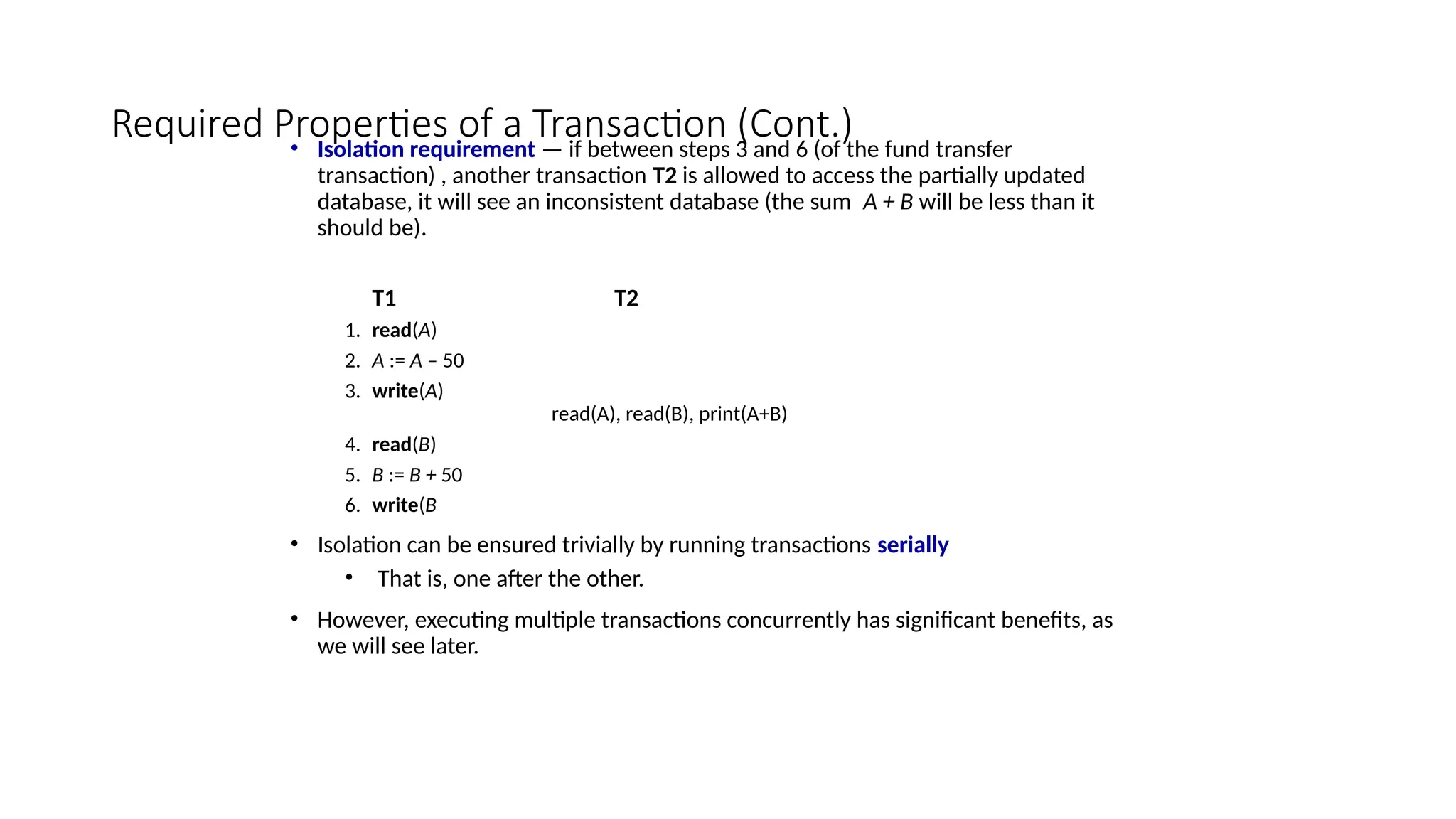
• Isolation requirement — if between steps 3 and 6 (of the fund transfer
transaction) , another transaction T2 is allowed to access the partially updated
database, it will see an inconsistent database (the sum A + B will be less than it
should be).
T1 T2
1. read(A)
2. A := A – 50
3. write(A)
read(A), read(B), print(A+B)
4. read(B)
5. B := B + 50
6. write(B
• Isolation can be ensured trivially by running transactions serially
• That is, one after the other.
• However, executing multiple transactions concurrently has significant benefits, as
we will see later.

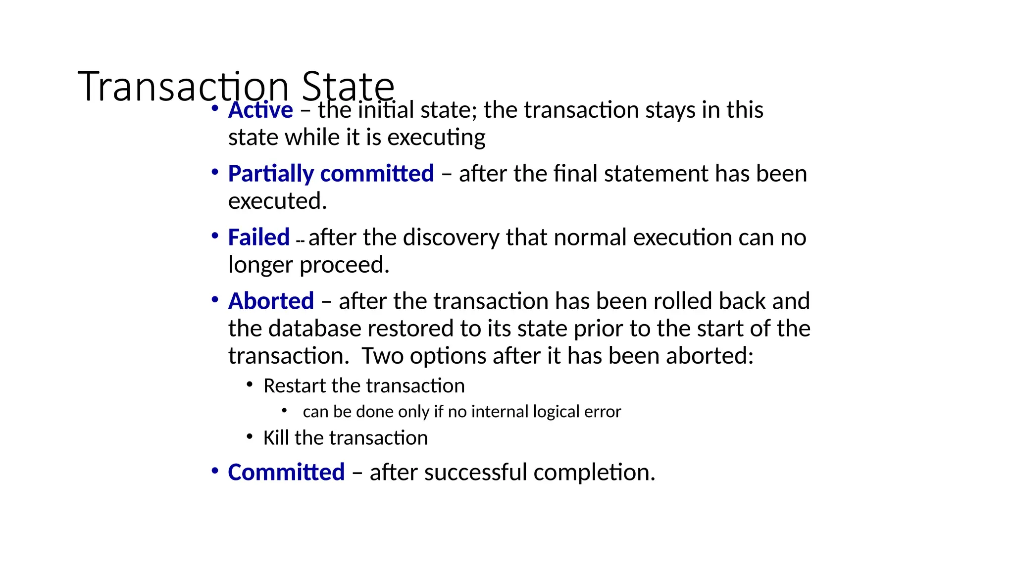
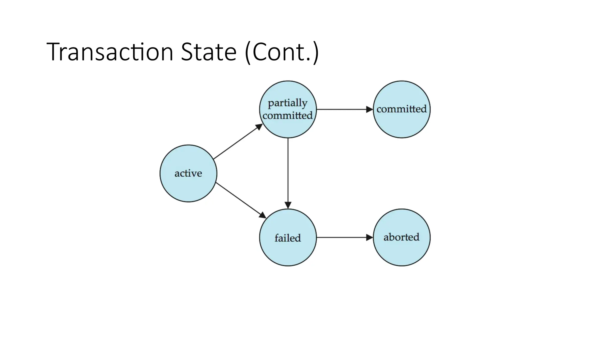
Transaction State
• Active – the initial state; the transaction stays in this
state while it is executing
• Partially committed – after the final statement has been
executed.
• Failed -- after the discovery that normal execution can no
longer proceed.
• Aborted – after the transaction has been rolled back and
the database restored to its state prior to the start of the
transaction. Two options after it has been aborted:
• Restart the transaction
• can be done only if no internal logical error
• Kill the transaction
• Committed – after successful completion.

Concurrent Executions
• Multiple transactions are allowed to run
concurrently in the system. Advantages are:
• Increased processor and disk utilization, leading
to better transaction throughput
• E.g. one transaction can be using the CPU while another
is reading from or writing to the disk
• Reduced average response time for transactions:
short transactions need not wait behind long ones.
• Concurrency control schemes – mechanisms
to achieve isolation
• That is, to control the interaction among the
concurrent transactions in order to prevent them
from destroying the consistency of the database

SERIALIZABILITY
Database System Concepts - 6th Edition 32.5 ©Silberschatz, Korth and Sudarshan
PPD
• Serializability
• Conflict
Serializabilit
y

Serializability
 Basic Assumption – Each transaction preserves database consistency
 Thus, serial execution of a set of transactions preserves database consistency
 A (possibly concurrent) schedule is serializable if it is equivalent to a serial schedule.
Different forms of schedule equivalence give rise to the notions of:
1. conflict serializability
2. view serializability

Simplified view of transactions
 We ignore operations other than read and write instructions
 Other operations happen in memory (are temporary in nature) and (mostly) do not
affect the state of the database
 This is a simplifying assumption for analysis
 We assume that transactions may perform arbitrary computations on data in local
buffers in between reads and writes
 Our simplified schedules consist of only read and write instructions

Conflicting Instructions
 Let li and lj be two Instructions of transactions Ti and Tj respectively. Instructions li and lj
conflict if and only if there exists some item Q accessed by both li and lj, and at least one of
these instructions wrote Q
1. li = read(Q), lj = read(Q). li and lj don’t conflict
2. li = read(Q), lj = write(Q). They conflict
3. li = write(Q), lj = read(Q). They conflict
4. li = write(Q), lj = write(Q). They conflict
 Intuitively, a conflict between li and lj forces a (logical) temporal order between them
 If li and lj are consecutive in a schedule and they do not conflict, their results would
remain the same even if they had been interchanged in the schedule

CONFLICT SERIALIZABILITY
PPD
• Serializability
• Conflict
Serializability

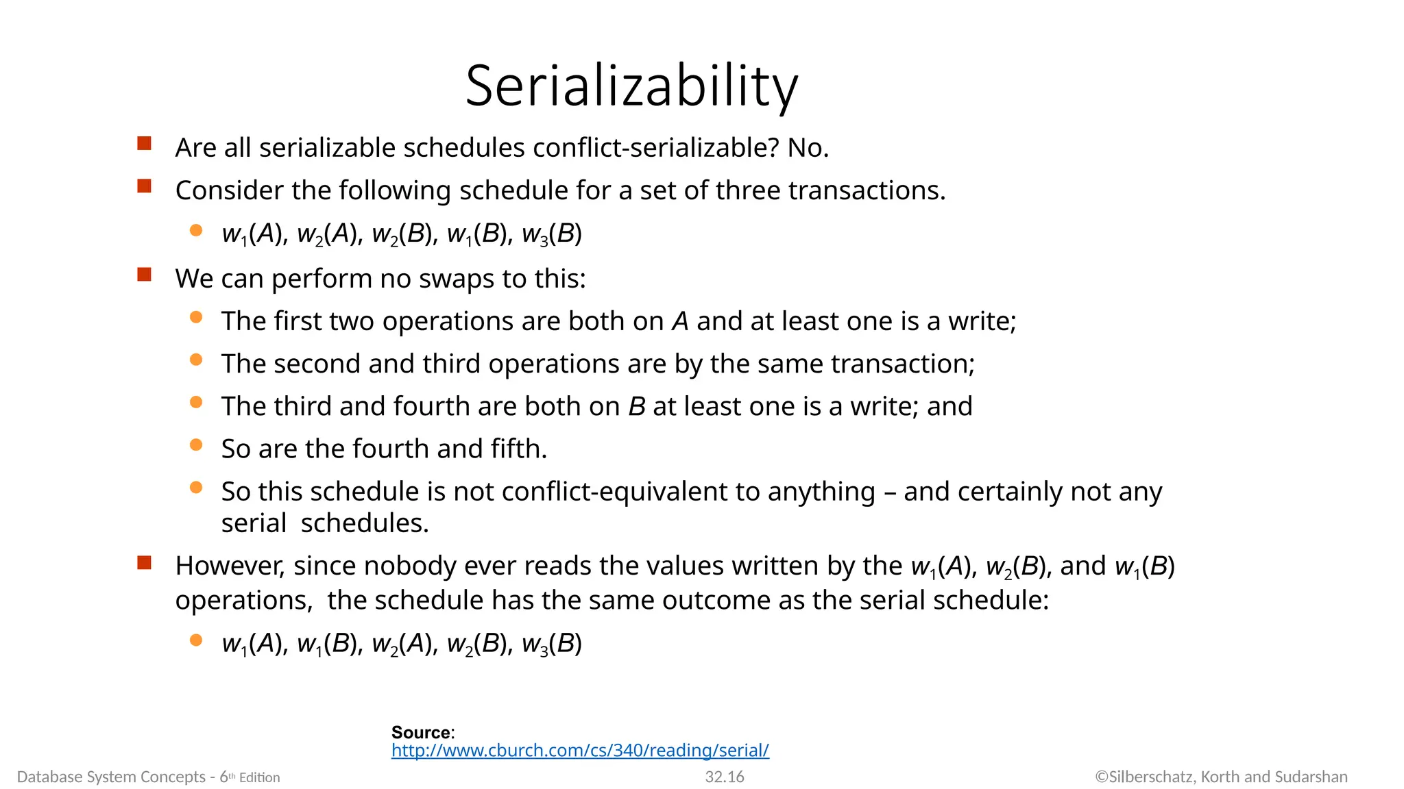
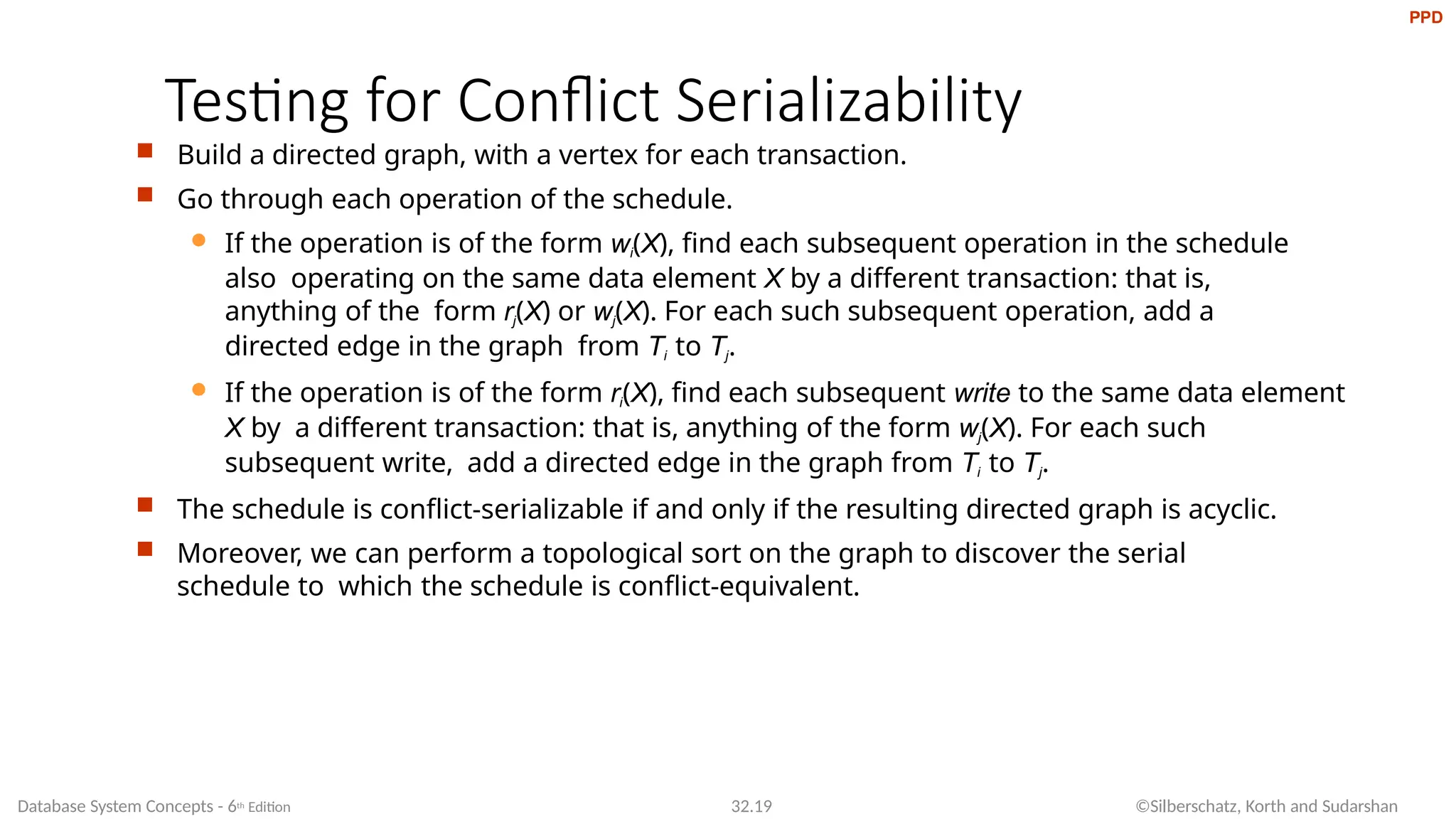
Conflict Serializability
 If a schedule S can be transformed into a schedule S’ by a series of swaps of non-
conflicting instructions, we say that S and S’ are conflict equivalent
 We say that a schedule S is conflict serializable if it is conflict equivalent to a serial
schedule

Conflict Serializability (Cont.)
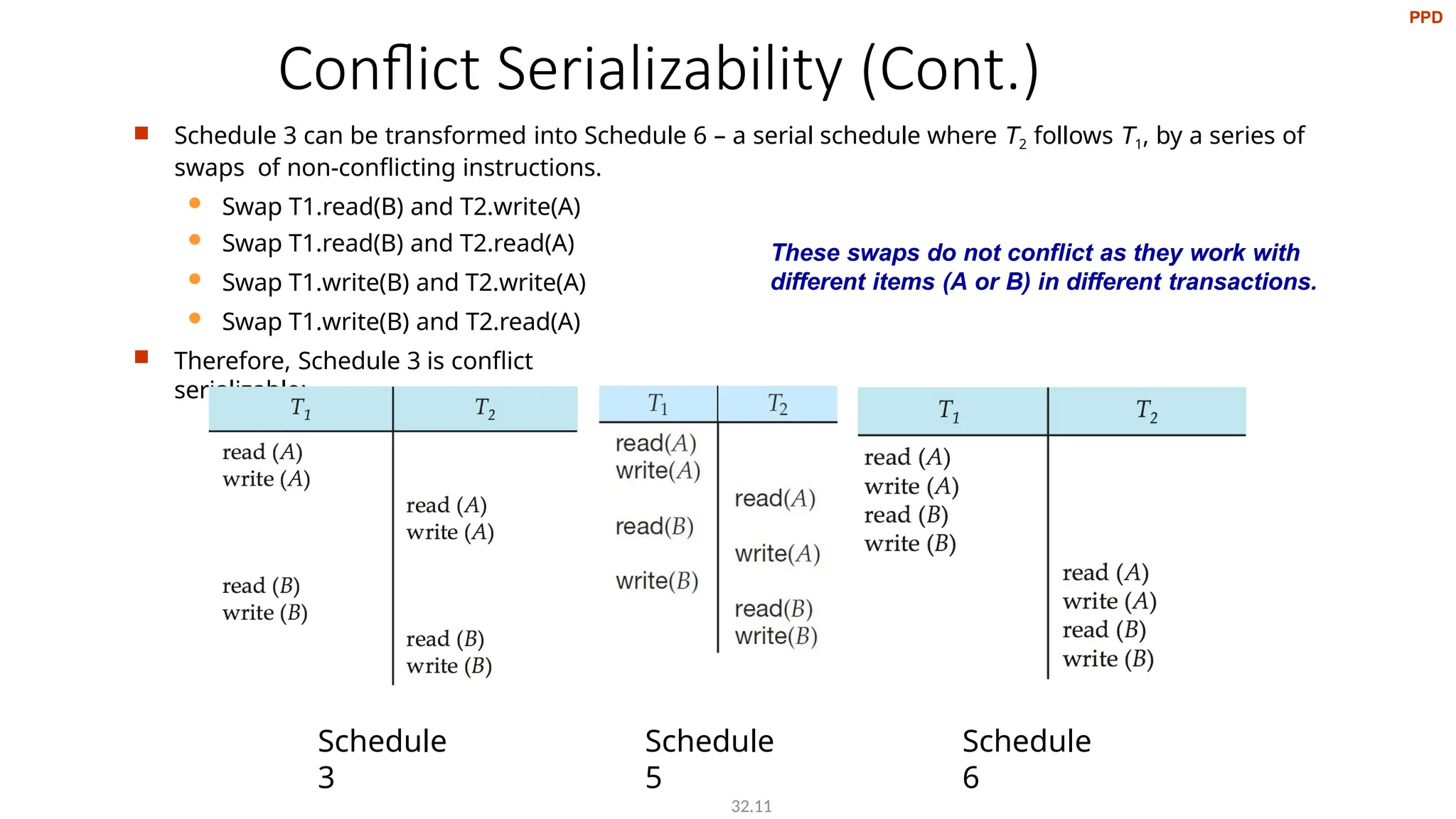
 Schedule 3 can be transformed into Schedule 6 – a serial schedule where T2 follows T1, by a series of
swaps of non-conflicting instructions.
 Swap T1.read(B) and T2.write(A)
 Swap T1.read(B) and T2.read(A)
 Swap T1.write(B) and T2.write(A)
 Swap T1.write(B) and T2.read(A)
 Therefore, Schedule 3 is conflict
serializable:
Schedule
3
Schedule
6
Schedule
5
32.11
PPD
These swaps do not conflict as they work with
different items (A or B) in different transactions.

Conflict Serializability (Cont.)
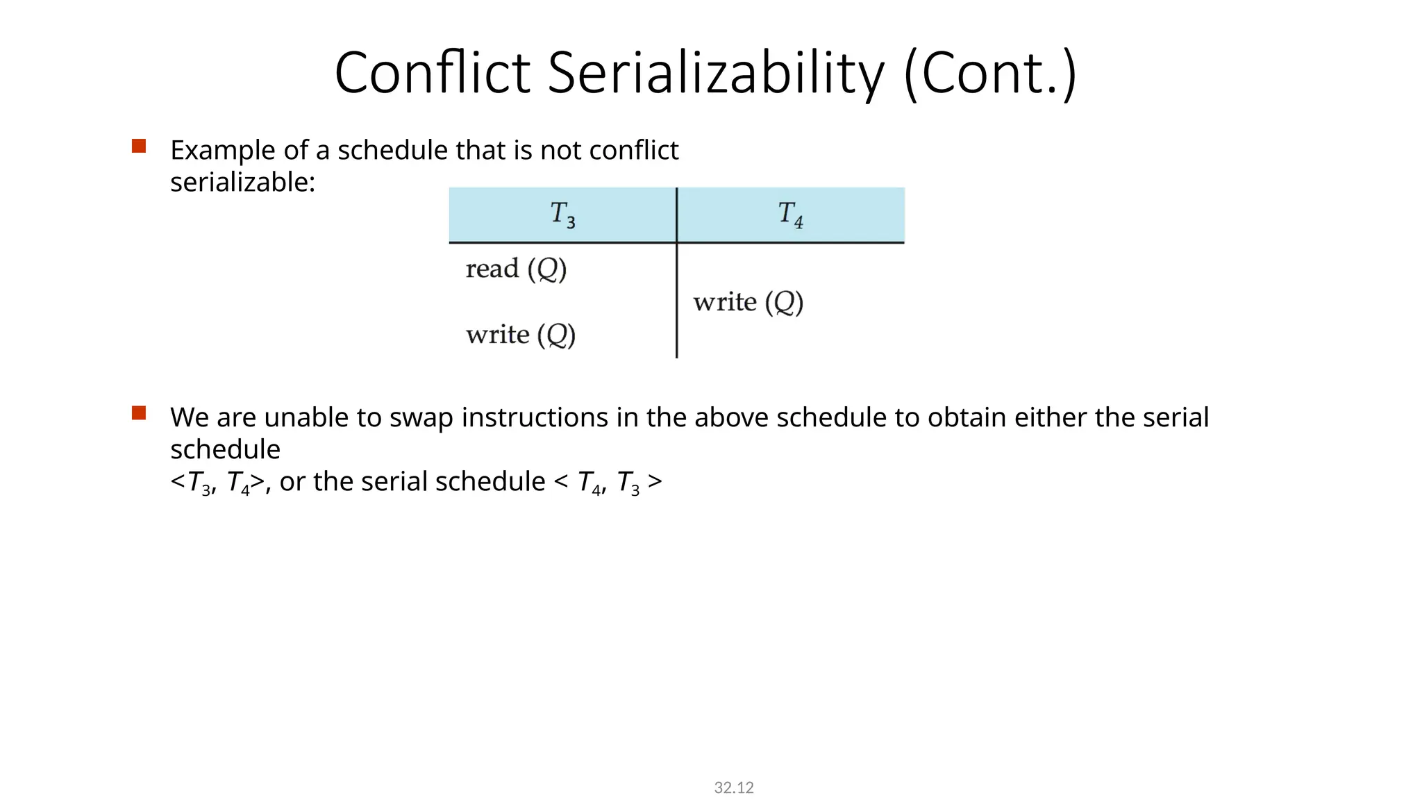
 Example of a schedule that is not conflict
serializable:
 We are unable to swap instructions in the above schedule to obtain either the serial
schedule
<T3, T4>, or the serial schedule < T4, T3 >
32.12

Example: Bad Schedule
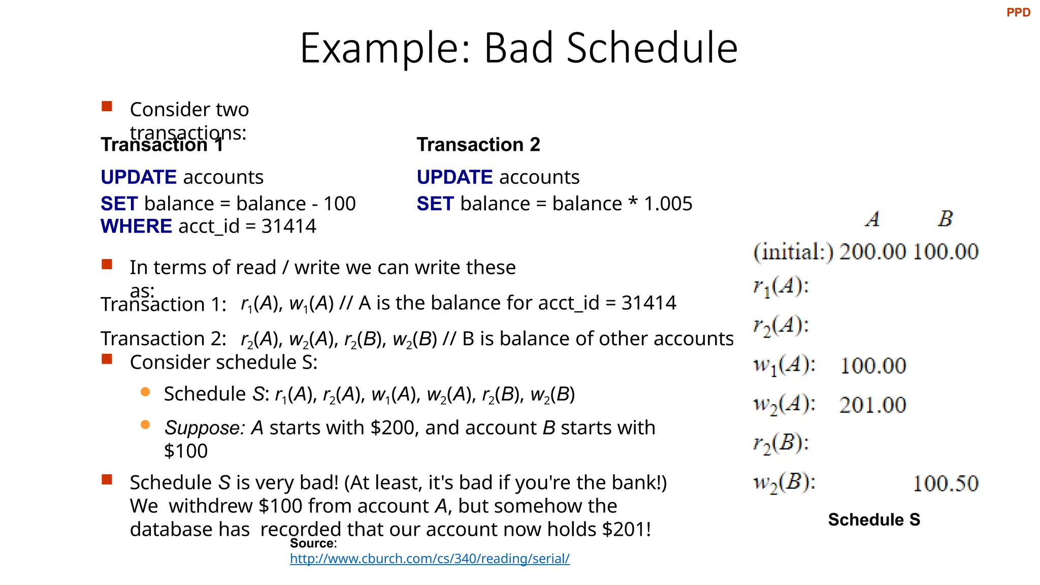
 Consider two
transactions:
 In terms of read / write we can write these
as:
 Consider schedule S:
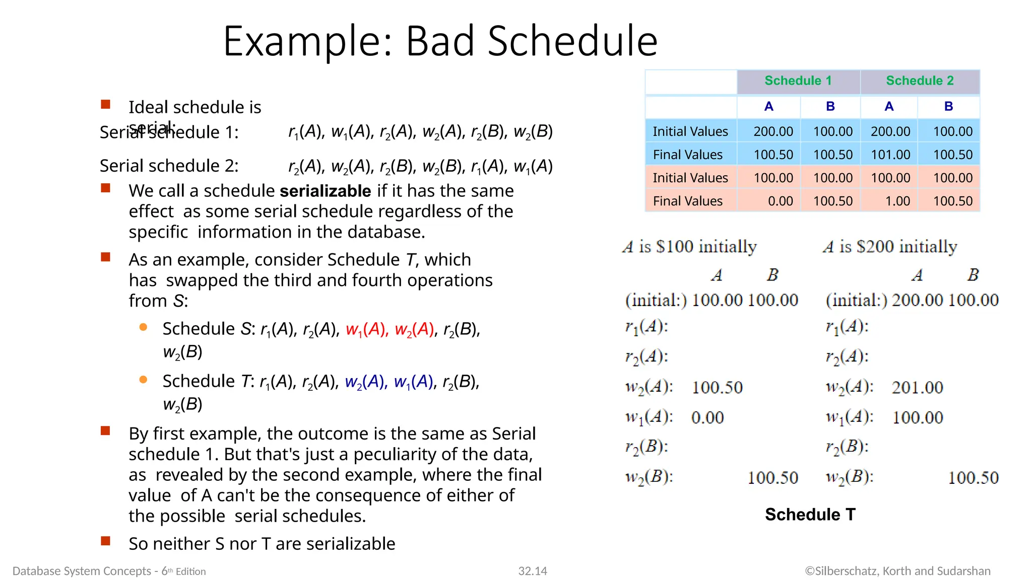
 Schedule S: r1(A), r2(A), w1(A), w2(A), r2(B), w2(B)
 Suppose: A starts with $200, and account B starts with
$100
 Schedule S is very bad! (At least, it's bad if you're the bank!)
We withdrew $100 from account A, but somehow the
database has recorded that our account now holds $201!
Transaction 1 Transaction 2
UPDATE accounts
SET balance = balance - 100
WHERE acct_id = 31414
UPDATE accounts
SET balance = balance * 1.005
Transaction 1: r1(A), w1(A) // A is the balance for acct_id = 31414
Transaction 2: r2(A), w2(A), r2(B), w2(B) // B is balance of other accounts
Schedule S
Source:
http://www.cburch.com/cs/340/reading/serial/
PPD

Example: Bad Schedule
 Ideal schedule is
serial:
 We call a schedule serializable if it has the same
effect as some serial schedule regardless of the
specific information in the database.
 As an example, consider Schedule T, which
has swapped the third and fourth operations
from S:
 Schedule S: r1(A), r2(A), w1(A), w2(A), r2(B),
w2(B)
 Schedule T: r1(A), r2(A), w2(A), w1(A), r2(B),
w2(B)
 By first example, the outcome is the same as Serial
schedule 1. But that's just a peculiarity of the data,
as revealed by the second example, where the final
value of A can't be the consequence of either of
the possible serial schedules.
 So neither S nor T are serializable
Serial schedule 1: r1(A), w1(A), r2(A), w2(A), r2(B), w2(B)
Serial schedule 2: r2(A), w2(A), r2(B), w2(B), r1(A), w1(A)
Schedule T
Schedule 1 Schedule 2
A B A B
Initial Values 200.00 100.00 200.00 100.00
Final Values 100.50 100.50 101.00 100.50
Initial Values 100.00 100.00 100.00 100.00
Final Values 0.00 100.50 1.00 100.50

Example: Good Schedule
32.15
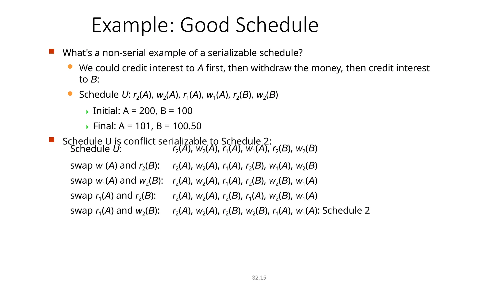
 What's a non-serial example of a serializable schedule?
 We could credit interest to A first, then withdraw the money, then credit interest
to B:
 Schedule U: r2(A), w2(A), r1(A), w1(A), r2(B), w2(B)
 Initial: A = 200, B = 100
 Final: A = 101, B = 100.50
 Schedule U is conflict serializable to Schedule 2:
Schedule U: r2(A), w2(A), r1(A), w1(A), r2(B), w2(B)
swap w1(A) and r2(B): r2(A), w2(A), r1(A), r2(B), w1(A), w2(B)
swap w1(A) and w2(B): r2(A), w2(A), r1(A), r2(B), w2(B), w1(A)
swap r1(A) and r2(B): r2(A), w2(A), r2(B), r1(A), w2(B), w1(A)
swap r1(A) and w2(B): r2(A), w2(A), r2(B), w2(B), r1(A), w1(A): Schedule 2

Serializability
Source:
 Are all serializable schedules conflict-serializable? No.
 Consider the following schedule for a set of three transactions.
 w1(A), w2(A), w2(B), w1(B), w3(B)
 We can perform no swaps to this:
 The first two operations are both on A and at least one is a write;
 The second and third operations are by the same transaction;
 The third and fourth are both on B at least one is a write; and
 So are the fourth and fifth.
 So this schedule is not conflict-equivalent to anything – and certainly not any
serial schedules.
 However, since nobody ever reads the values written by the w1(A), w2(B), and w1(B)
operations, the schedule has the same outcome as the serial schedule:
 w1(A), w1(B), w2(A), w2(B), w3(B)

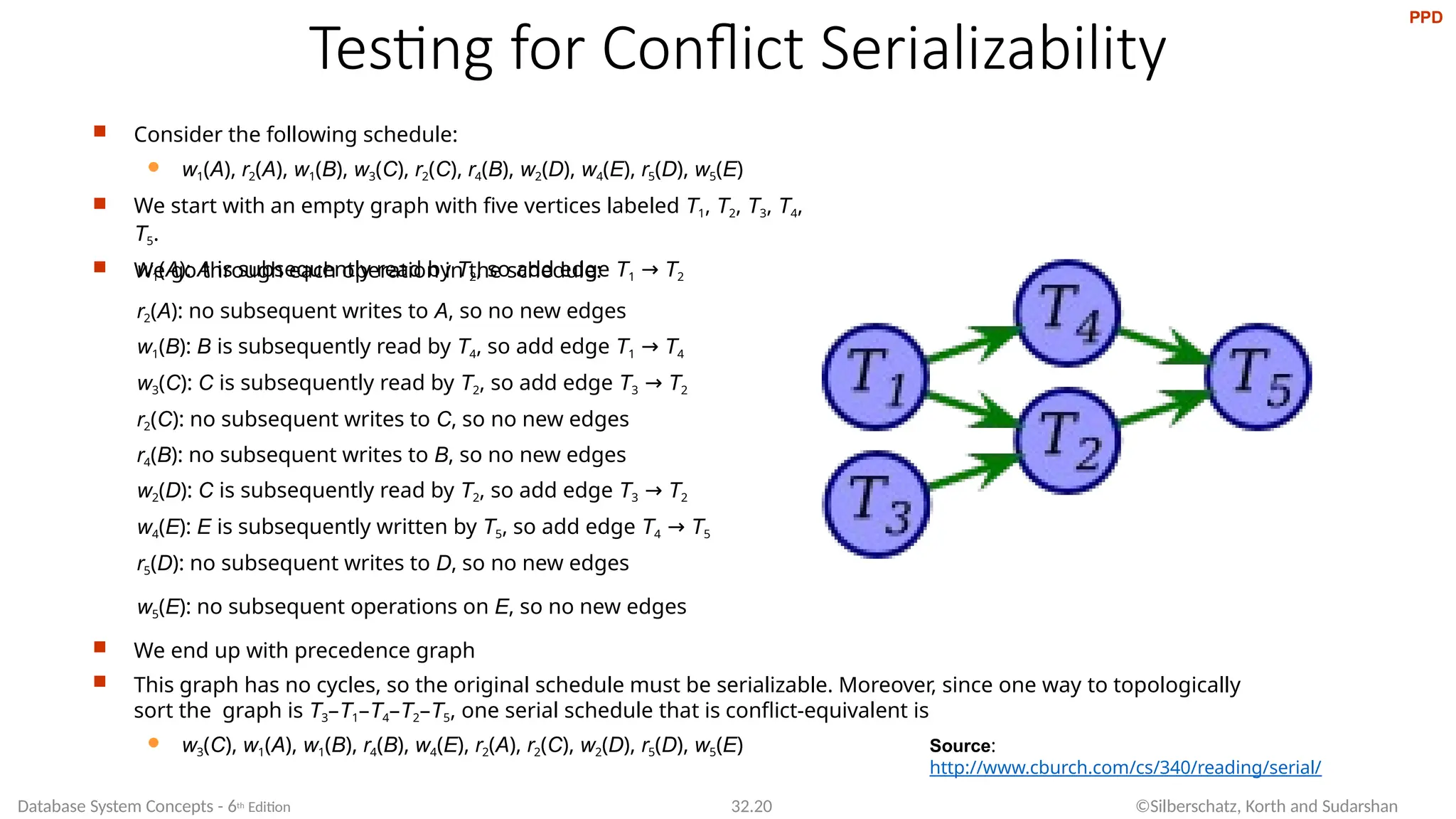
Precedence Graph
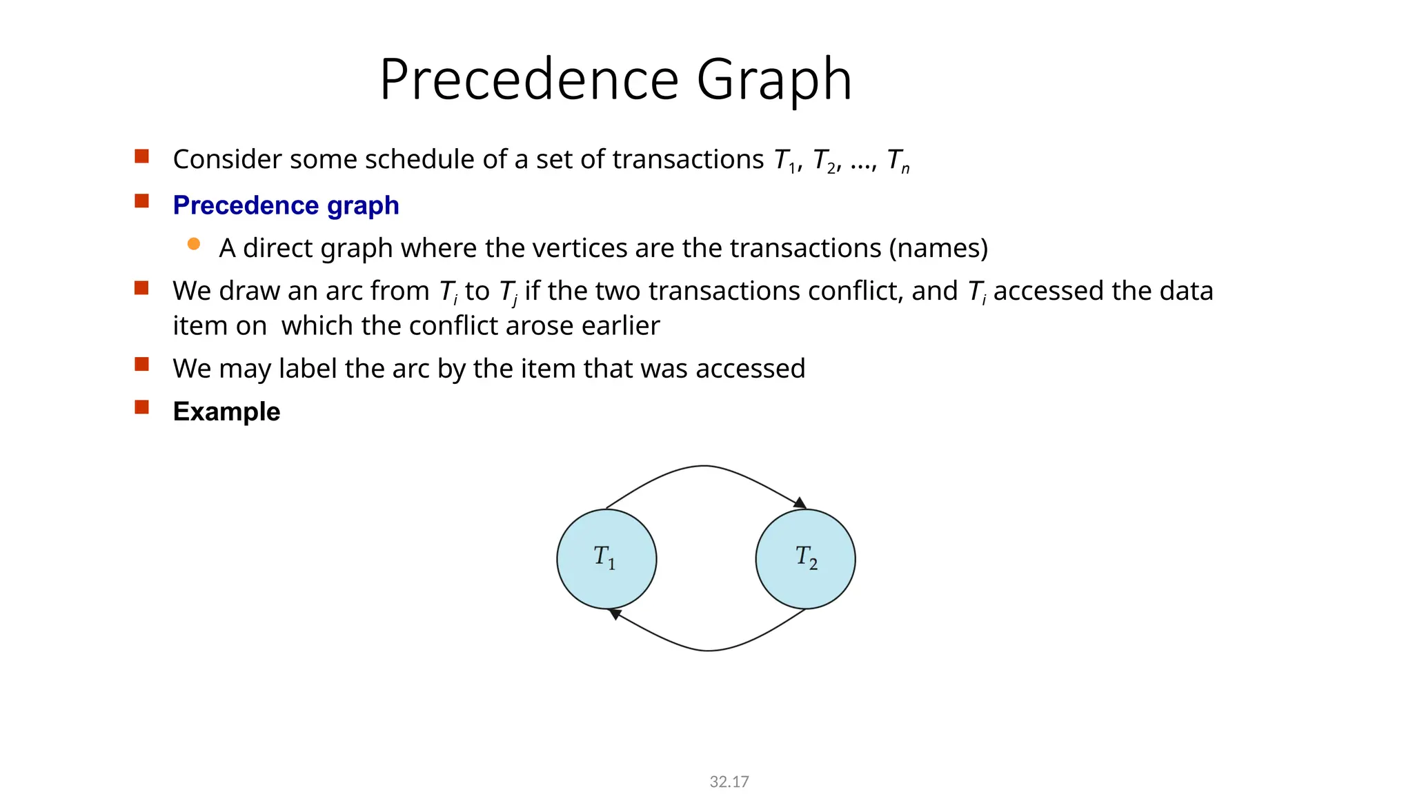
 Consider some schedule of a set of transactions T1, T2, ..., Tn
 Precedence graph
 A direct graph where the vertices are the transactions (names)
 We draw an arc from Ti to Tj if the two transactions conflict, and Ti accessed the data
item on which the conflict arose earlier
 We may label the arc by the item that was accessed
 Example
32.17

Testing for Conflict Serializability
 A schedule is conflict serializable if and only if its precedence graph is
acyclic
 Cycle-detection algorithms exist which take order n2 time, where n is
the number of vertices in the graph
 (Better algorithms take order n + e where e is the number of
edges.)
 If precedence graph is acyclic, the serializability order can be
obtained by a
topological sorting of the graph
 That is, a linear order consistent with the partial order of the
graph.
 For example, a serializability order for the schedule (a) would be
one of either (b) or (c)

 Build a directed graph, with a vertex for each transaction.
 Go through each operation of the schedule.
 If the operation is of the form wi(X), find each subsequent operation in the schedule
also operating on the same data element X by a different transaction: that is,
anything of the form rj(X) or wj(X). For each such subsequent operation, add a
directed edge in the graph from Ti to Tj.
 If the operation is of the form ri(X), find each subsequent write to the same data element
X by a different transaction: that is, anything of the form wj(X). For each such
subsequent write, add a directed edge in the graph from Ti to Tj.
 The schedule is conflict-serializable if and only if the resulting directed graph is acyclic.
 Moreover, we can perform a topological sort on the graph to discover the serial
schedule to which the schedule is conflict-equivalent.
PPD

 Consider the following schedule:
 w1(A), r2(A), w1(B), w3(C), r2(C), r4(B), w2(D), w4(E), r5(D), w5(E)
 We start with an empty graph with five vertices labeled T1, T2, T3, T4,
T5.
 We go through each operation in the schedule:
 We end up with precedence graph
 This graph has no cycles, so the original schedule must be serializable. Moreover, since one way to topologically
sort the graph is T3–T1–T4–T2–T5, one serial schedule that is conflict-equivalent is
 w3(C), w1(A), w1(B), r4(B), w4(E), r2(A), r2(C), w2(D), r5(D), w5(E)
w1(A): A is subsequently read by T2, so add edge T1 → T2
r2(A): no subsequent writes to A, so no new edges
w1(B): B is subsequently read by T4, so add edge T1 → T4
w3(C): C is subsequently read by T2, so add edge T3 → T2
r2(C): no subsequent writes to C, so no new edges
r4(B): no subsequent writes to B, so no new edges
w2(D): C is subsequently read by T2, so add edge T3 → T2
w4(E): E is subsequently written by T5, so add edge T4 → T5
r5(D): no subsequent writes to D, so no new edges
w5(E): no subsequent operations on E, so no new edges
Source:
PPD

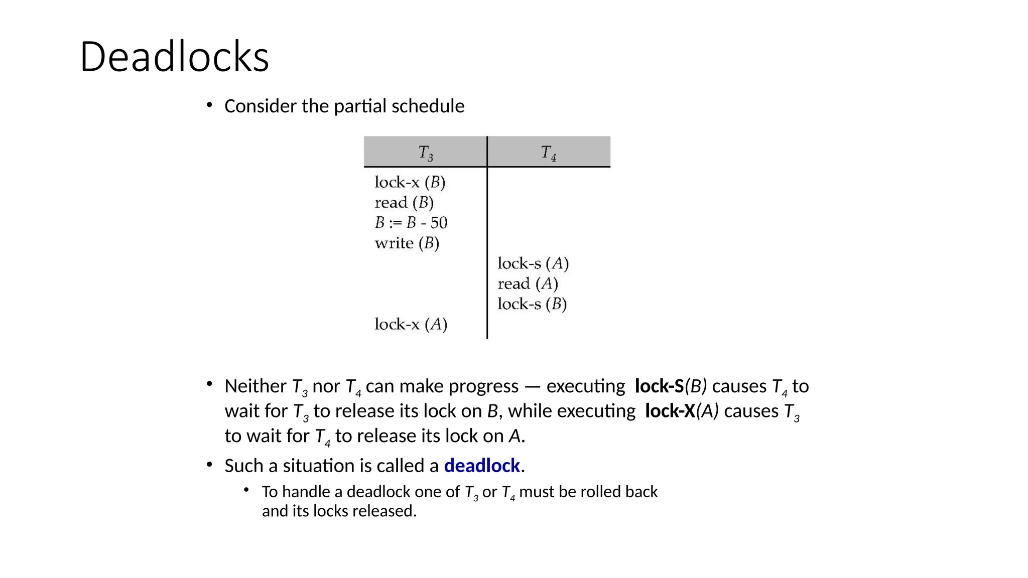
Deadlocks
• Consider the partial schedule
• Neither T3 nor T4 can make progress — executing lock-S(B) causes T4 to
wait for T3 to release its lock on B, while executing lock-X(A) causes T3
to wait for T4 to release its lock on A.
• Such a situation is called a deadlock.
• To handle a deadlock one of T3 or T4 must be rolled back
and its locks released.

Deadlocks (Cont.)
• Two-phase locking does not ensure freedom from
deadlocks.
• In addition to deadlocks, there is a possibility of
starvation.
• Starvation occurs if the concurrency control manager
is badly designed. For example:
• A transaction may be waiting for an X-lock on an item,
while a sequence of other transactions request and are
granted an S-lock on the same item.
• The same transaction is repeatedly rolled back due to
deadlocks.
• Concurrency control manager can be designed to
prevent starvation.

Deadlocks (Cont.)
• The potential for deadlock exists in most locking protocols.
Deadlocks are a necessary evil.
• When a deadlock occurs there is a possibility of cascading
roll-backs.
• Cascading roll-back is possible under two-phase locking. To
avoid this, follow a modified protocol called strict two-phase
locking -- a transaction must hold all its exclusive locks till it
commits/aborts.
• Rigorous two-phase locking is even stricter. Here, all locks are
held till commit/abort. In this protocol transactions can be
serialized in the order in which they commit.

Implementation of Locking
• A lock manager can be implemented as a separate
process to which transactions send lock and unlock
requests
• The lock manager replies to a lock request by sending a
lock grant messages (or a message asking the
transaction to roll back, in case of a deadlock)
• The requesting transaction waits until its request is
answered
• The lock manager maintains a data-structure called a
lock table to record granted locks and pending requests
• The lock table is usually implemented as an in-memory
hash table indexed on the name of the data item being
locked

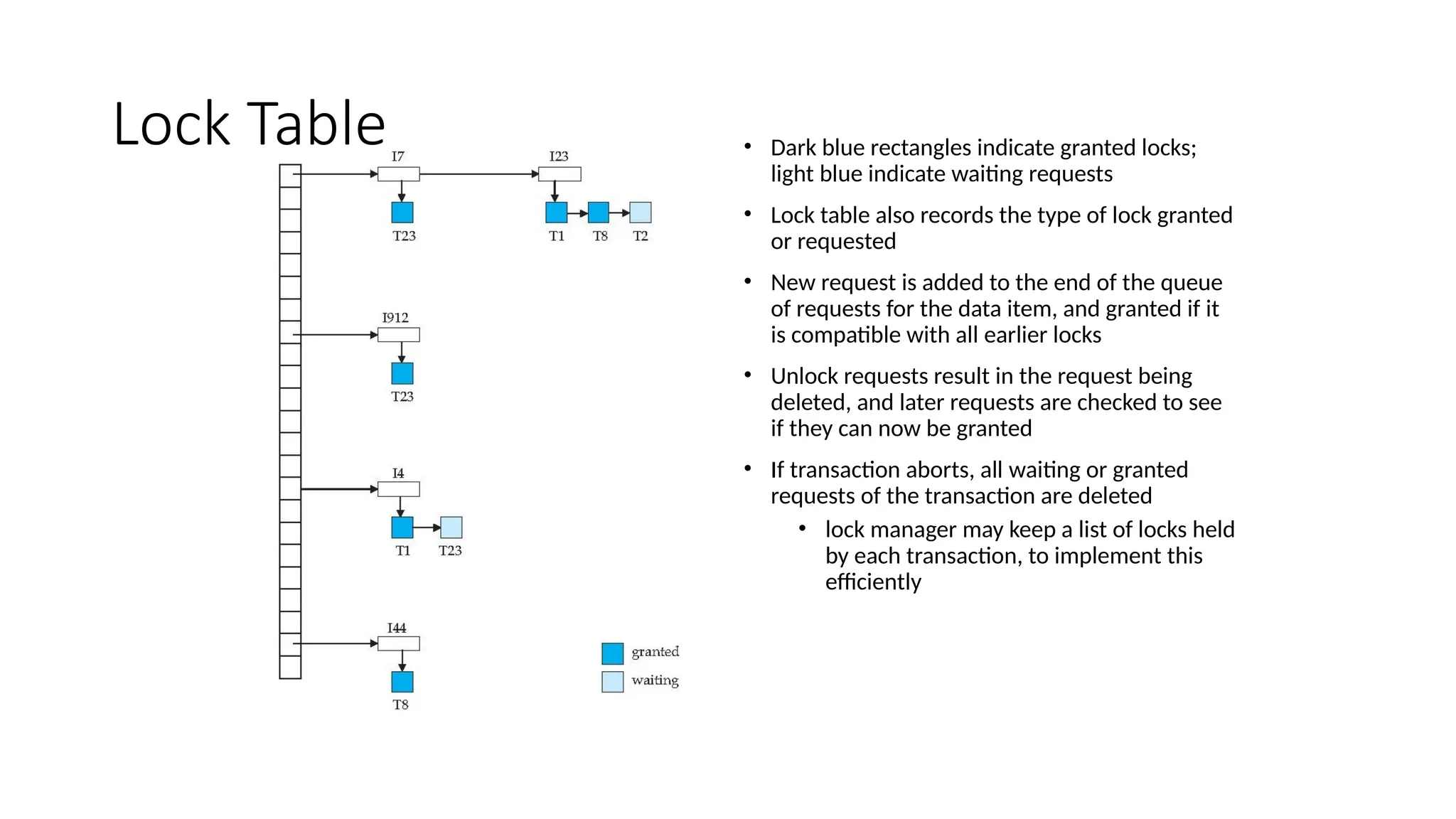
Lock Table • Dark blue rectangles indicate granted locks;
light blue indicate waiting requests
• Lock table also records the type of lock granted
or requested
• New request is added to the end of the queue
of requests for the data item, and granted if it
is compatible with all earlier locks
• Unlock requests result in the request being
deleted, and later requests are checked to see
if they can now be granted
• If transaction aborts, all waiting or granted
requests of the transaction are deleted
• lock manager may keep a list of locks held
by each transaction, to implement this
efficiently

Deadlock Handling
• System is deadlocked if there is a set of transactions such
that every transaction in the set is waiting for another
transaction in the set.
• Deadlock prevention protocols ensure that the system will
never enter into a deadlock state. Some prevention
strategies :
• Require that each transaction locks all its data items before it
begins execution (predeclaration).
• Impose partial ordering of all data items and require that a
transaction can lock data items only in the order specified by the
partial order.

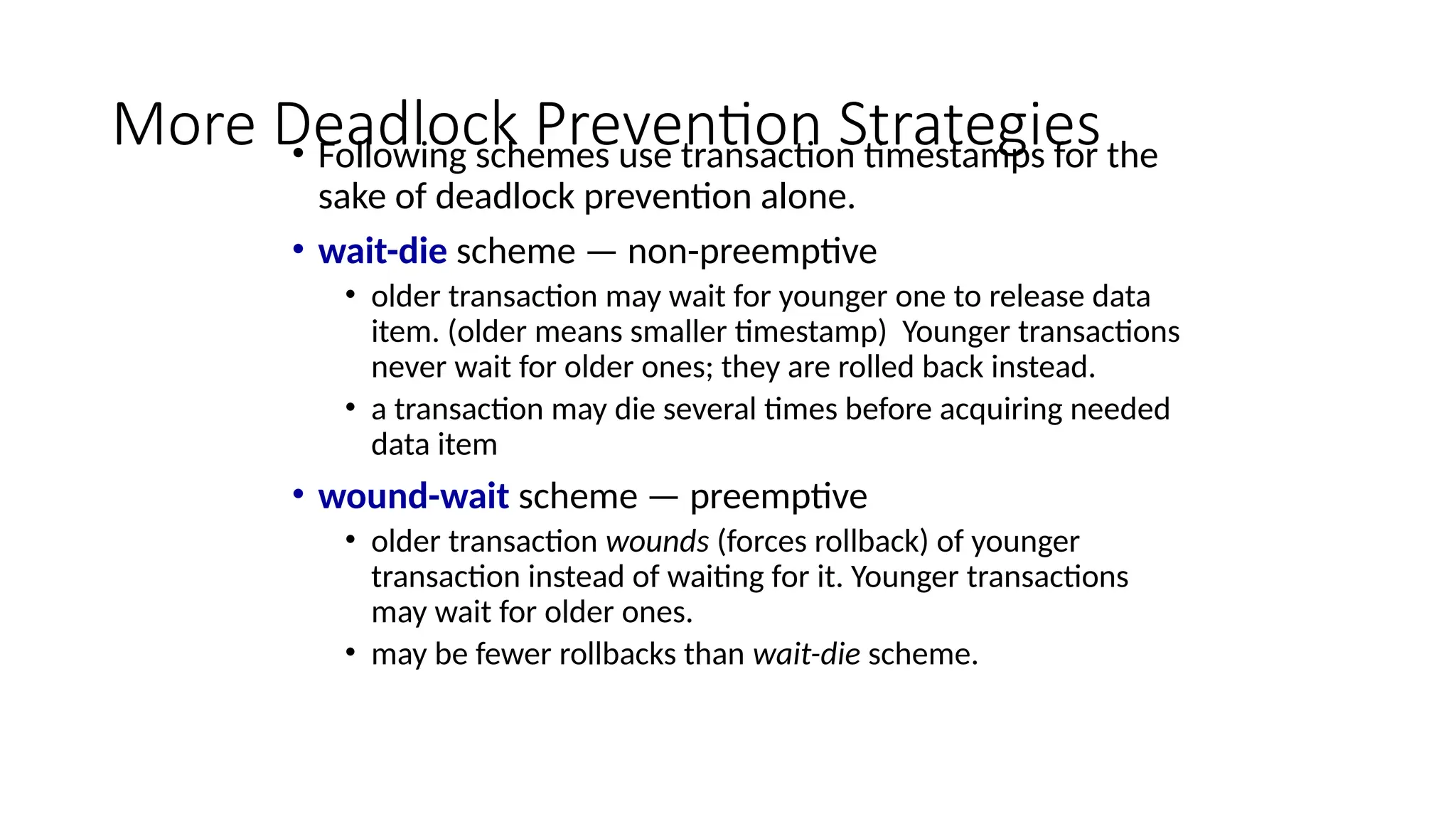
More Deadlock Prevention Strategies
• Following schemes use transaction timestamps for the
sake of deadlock prevention alone.
• wait-die scheme — non-preemptive
• older transaction may wait for younger one to release data
item. (older means smaller timestamp) Younger transactions
never wait for older ones; they are rolled back instead.
• a transaction may die several times before acquiring needed
data item
• wound-wait scheme — preemptive
• older transaction wounds (forces rollback) of younger
transaction instead of waiting for it. Younger transactions
may wait for older ones.
• may be fewer rollbacks than wait-die scheme.

Deadlock prevention (Cont.)
• Both in wait-die and in wound-wait schemes, a rolled back
transactions is restarted with its original timestamp. Older
transactions thus have precedence over newer ones, and starvation is
hence avoided.
• Timeout-Based Schemes:
• a transaction waits for a lock only for a specified amount of time. If the lock
has not been granted within that time, the transaction is rolled back and
restarted,
• Thus, deadlocks are not possible
• simple to implement; but starvation is possible. Also difficult to determine
good value of the timeout interval.

Deadlock Detection
• Deadlocks can be described as a wait-for graph, which consists of a pair G = (V,E),
• V is a set of vertices (all the transactions in the system)
• E is a set of edges; each element is an ordered pair Ti Tj.
• If Ti  Tj is in E, then there is a directed edge from Ti to Tj, implying that Ti is
waiting for Tj to release a data item.
• When Ti requests a data item currently being held by Tj, then the edge Ti  Tj is
inserted in the wait-for graph. This edge is removed only when Tj is no longer
holding a data item needed by Ti.
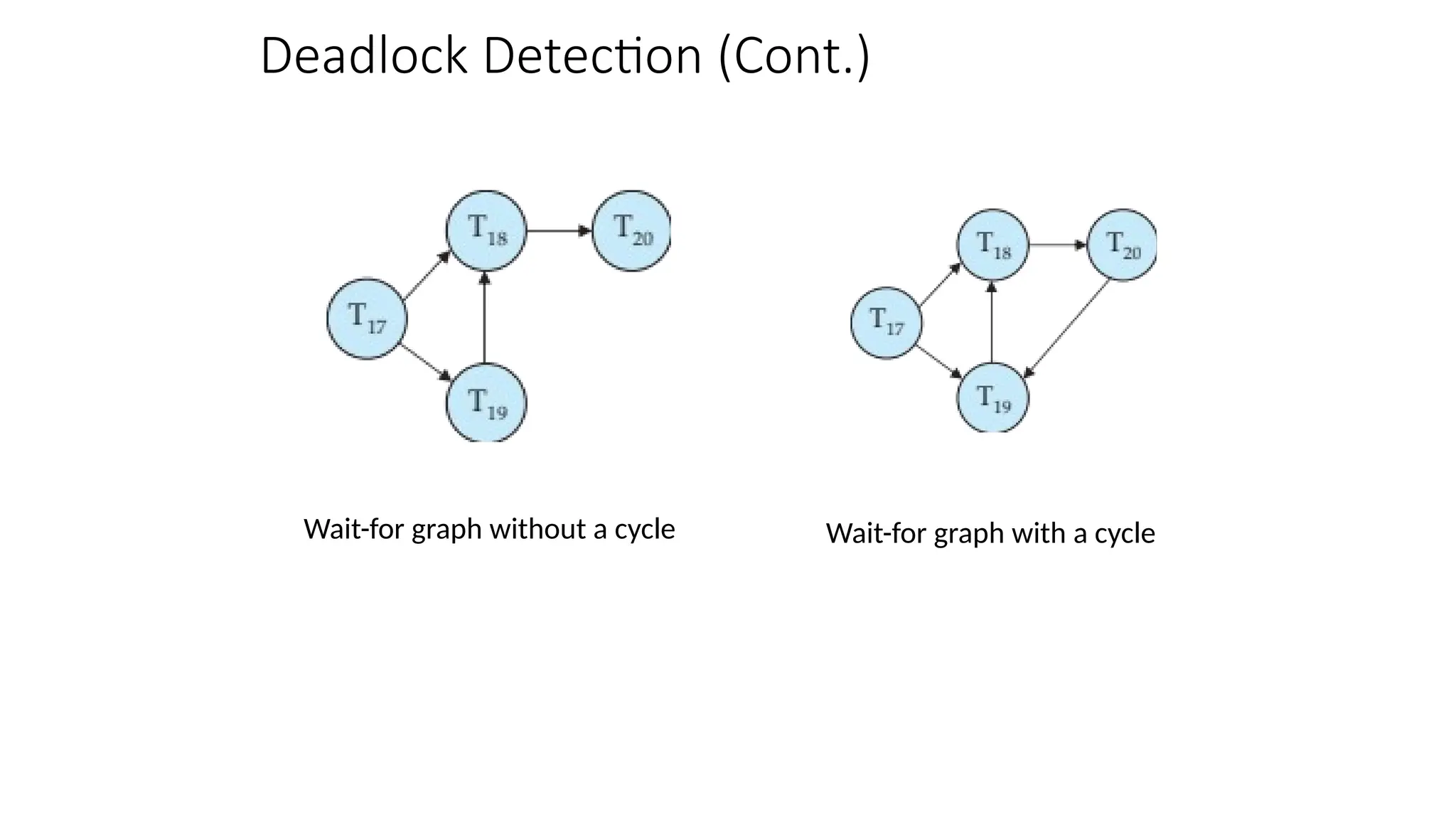
• The system is in a deadlock state if and only if the wait-for graph has a cycle.
Must invoke a deadlock-detection algorithm periodically to look for cycles.

Deadlock Detection (Cont.)
Wait-for graph without a cycle Wait-for graph with a cycle

Deadlock Recovery
• When deadlock is detected :
• Some transaction will have to rolled back (made a
victim) to break deadlock. Select that transaction as
victim that will incur minimum cost.
• Rollback -- determine how far to roll back
transaction
• Total rollback: Abort the transaction and then restart it.
• More effective to roll back transaction only as far as
necessary to break deadlock.
• Starvation happens if same transaction is always
chosen as victim. Include the number of rollbacks in
the cost factor to avoid starvation

Multiple Granularity
• Allow data items to be of various sizes and define a hierarchy of data
granularities, where the small granularities are nested within larger
ones
• Can be represented graphically as a tree.
• When a transaction locks a node in the tree explicitly, it implicitly
locks all the node's descendents in the same mode.
• Granularity of locking (level in tree where locking is done):
• fine granularity (lower in tree): high concurrency, high locking overhead
• coarse granularity (higher in tree): low locking overhead, low concurrency

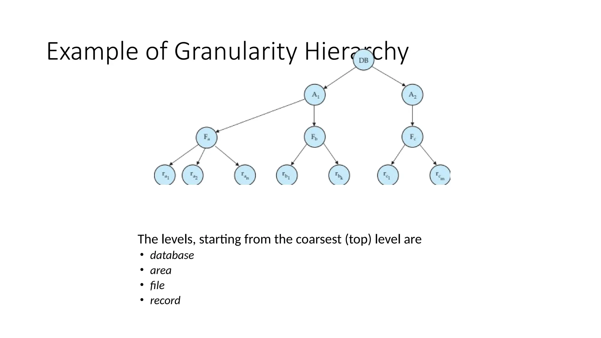
Example of Granularity Hierarchy
The levels, starting from the coarsest (top) level are
• database
• area
• file
• record

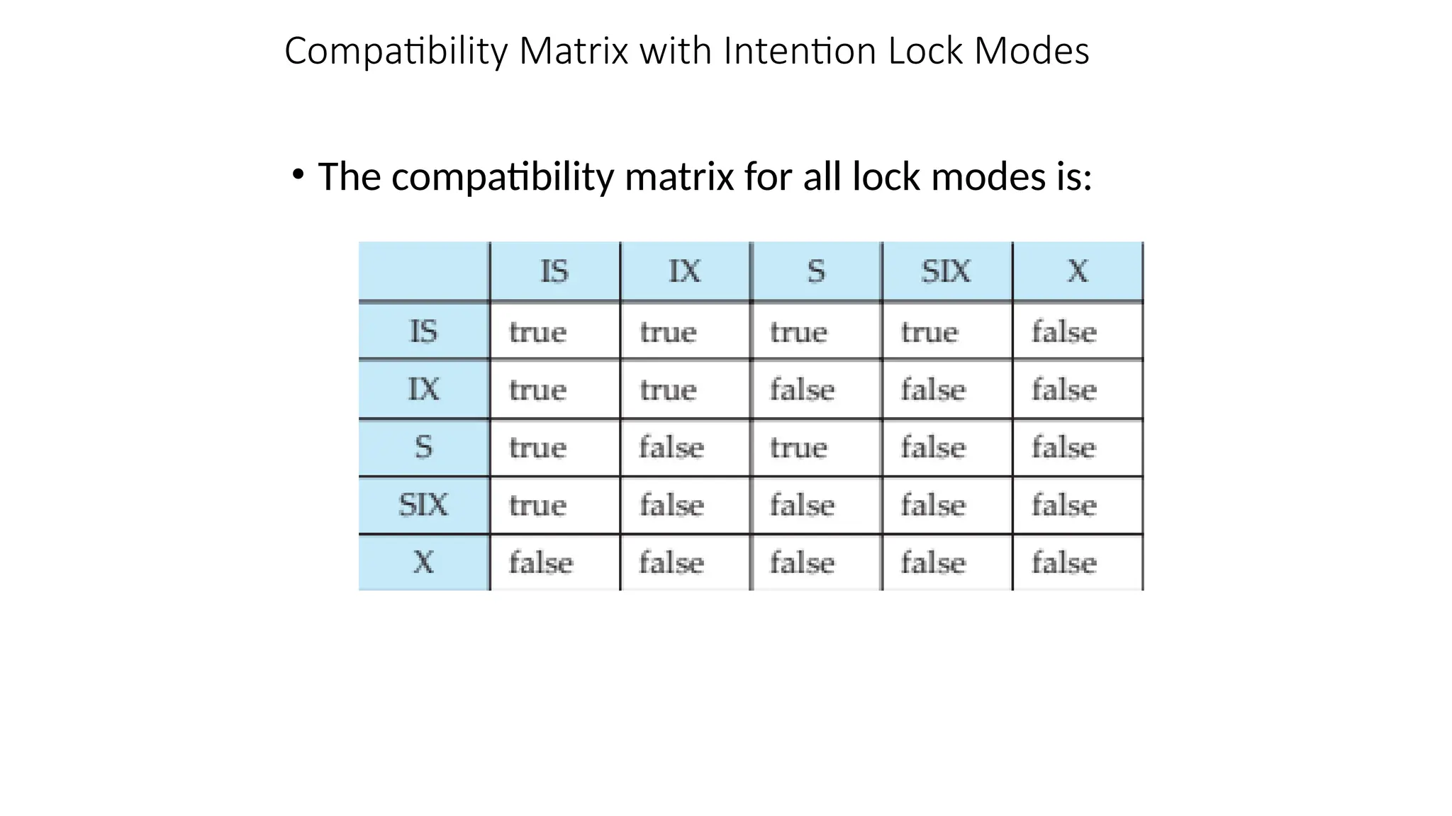
Intention Lock Modes
• In addition to S and X lock modes, there are three additional lock
modes with multiple granularity:
• intention-shared (IS): indicates explicit locking at a lower level of the tree but
only with shared locks.
• intention-exclusive (IX): indicates explicit locking at a lower level with
exclusive or shared locks
• shared and intention-exclusive (SIX): the subtree rooted by that node is
locked explicitly in shared mode and explicit locking is being done at a lower
level with exclusive-mode locks.
• intention locks allow a higher level node to be locked in S or X mode
without having to check all descendent nodes.

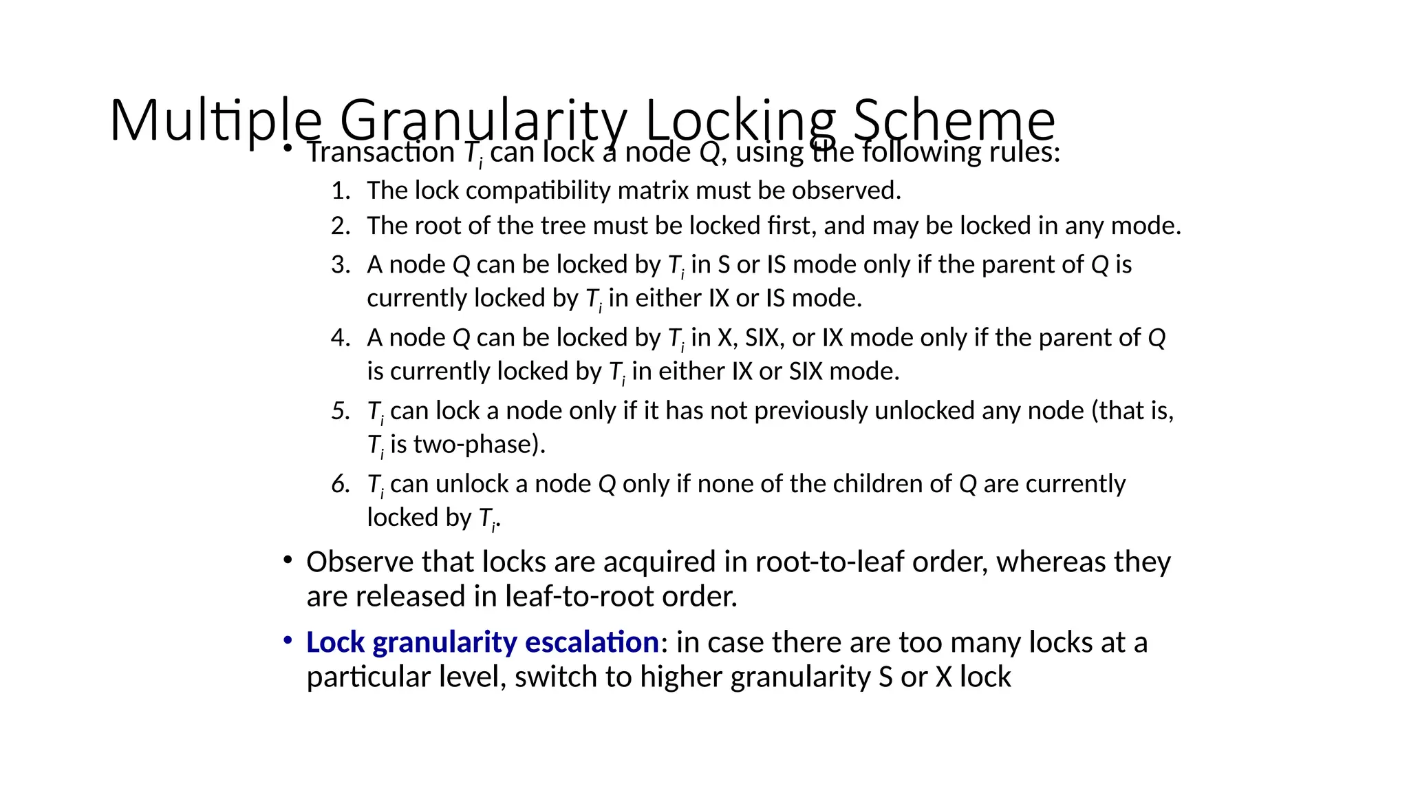
Compatibility Matrix with Intention Lock Modes
• The compatibility matrix for all lock modes is:

Multiple Granularity Locking Scheme
• Transaction Ti can lock a node Q, using the following rules:
1. The lock compatibility matrix must be observed.
2. The root of the tree must be locked first, and may be locked in any mode.
3. A node Q can be locked by Ti in S or IS mode only if the parent of Q is
currently locked by Ti in either IX or IS mode.
4. A node Q can be locked by Ti in X, SIX, or IX mode only if the parent of Q
is currently locked by Ti in either IX or SIX mode.
5. Ti can lock a node only if it has not previously unlocked any node (that is,
Ti is two-phase).
6. Ti can unlock a node Q only if none of the children of Q are currently
locked by Ti.
• Observe that locks are acquired in root-to-leaf order, whereas they
are released in leaf-to-root order.
• Lock granularity escalation: in case there are too many locks at a
particular level, switch to higher granularity S or X lock

RECOVERABILITY AND ISOLATION
PPD
• Recoverability and
Isolation
• Transaction
Definition in
SQL
• View
Serializability
• Complex Notions
of Serializability

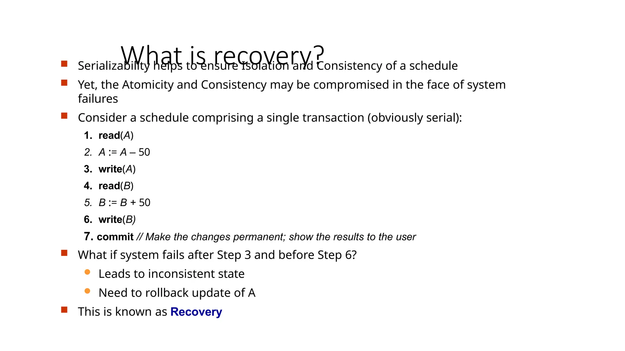
What is recovery?
 Serializability helps to ensure Isolation and Consistency of a schedule
 Yet, the Atomicity and Consistency may be compromised in the face of system
failures
 Consider a schedule comprising a single transaction (obviously serial):
1. read(A)
2. A := A – 50
3. write(A)
4. read(B)
5. B := B + 50
6. write(B)
7. commit // Make the changes permanent; show the results to the user
 What if system fails after Step 3 and before Step 6?
 Leads to inconsistent state
 Need to rollback update of A
 This is known as Recovery

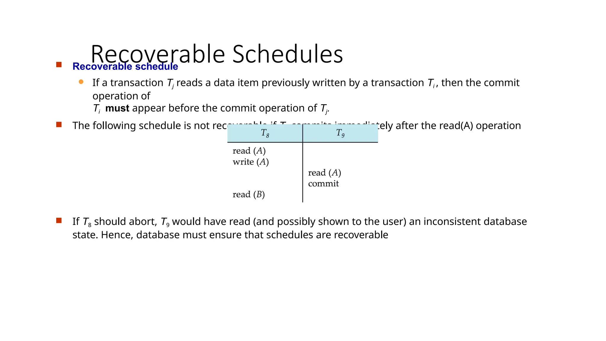
Recoverable Schedules
 Recoverable schedule
 If a transaction Tj reads a data item previously written by a transaction Ti , then the commit
operation of
Ti must appear before the commit operation of Tj.
 The following schedule is not recoverable if T9 commits immediately after the read(A) operation
 If T8 should abort, T9 would have read (and possibly shown to the user) an inconsistent database
state. Hence, database must ensure that schedules are recoverable

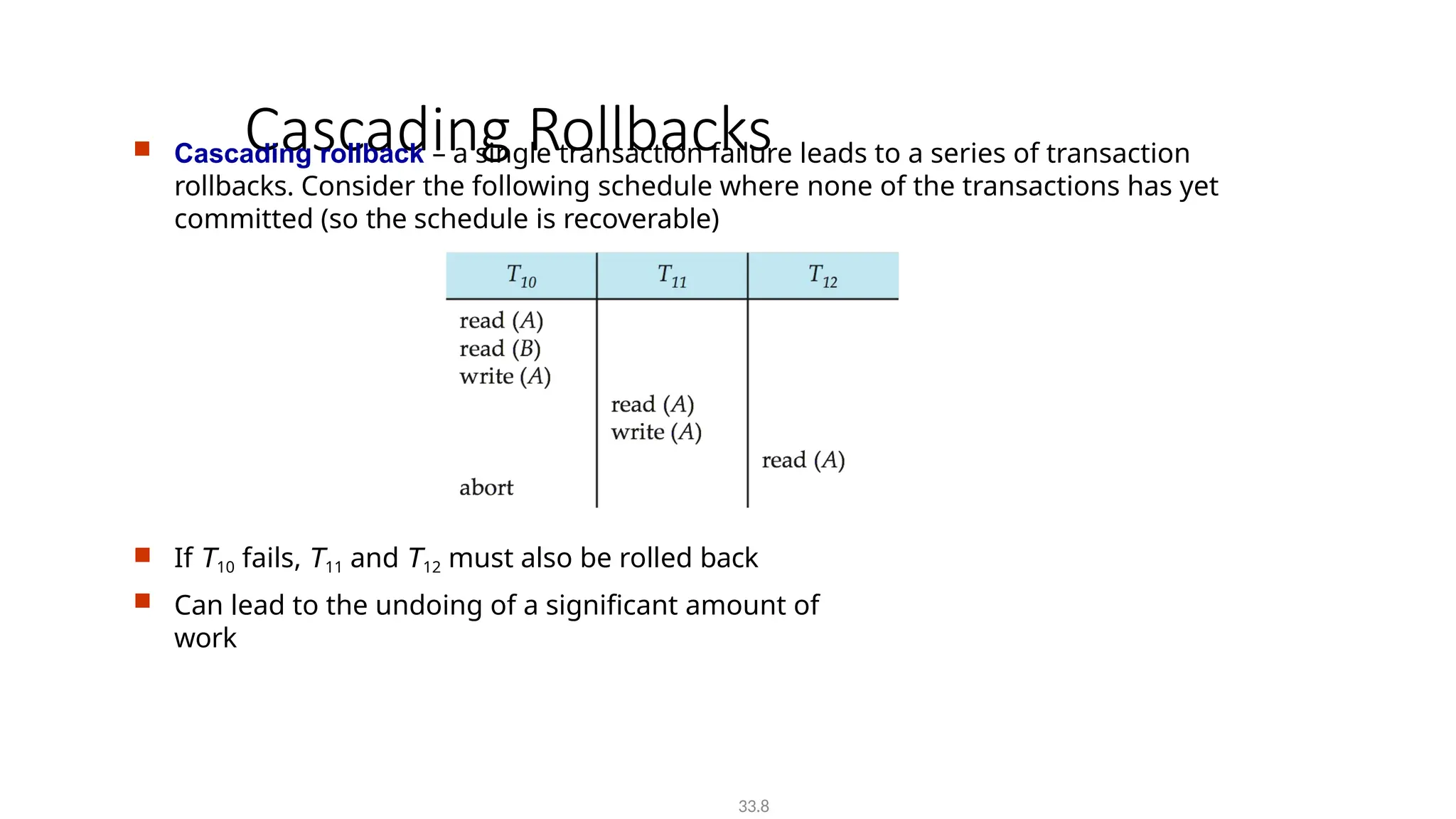
Cascading Rollbacks
 Cascading rollback – a single transaction failure leads to a series of transaction
rollbacks. Consider the following schedule where none of the transactions has yet
committed (so the schedule is recoverable)
 If T10 fails, T11 and T12 must also be rolled back
 Can lead to the undoing of a significant amount of
work
33.8

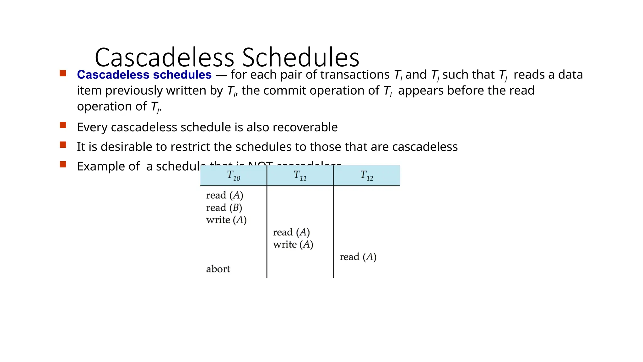
Cascadeless Schedules
 Cascadeless schedules — for each pair of transactions Ti and Tj such that Tj reads a data
item previously written by Ti, the commit operation of Ti appears before the read
operation of Tj.
 Every cascadeless schedule is also recoverable
 It is desirable to restrict the schedules to those that are cascadeless
 Example of a schedule that is NOT cascadeless

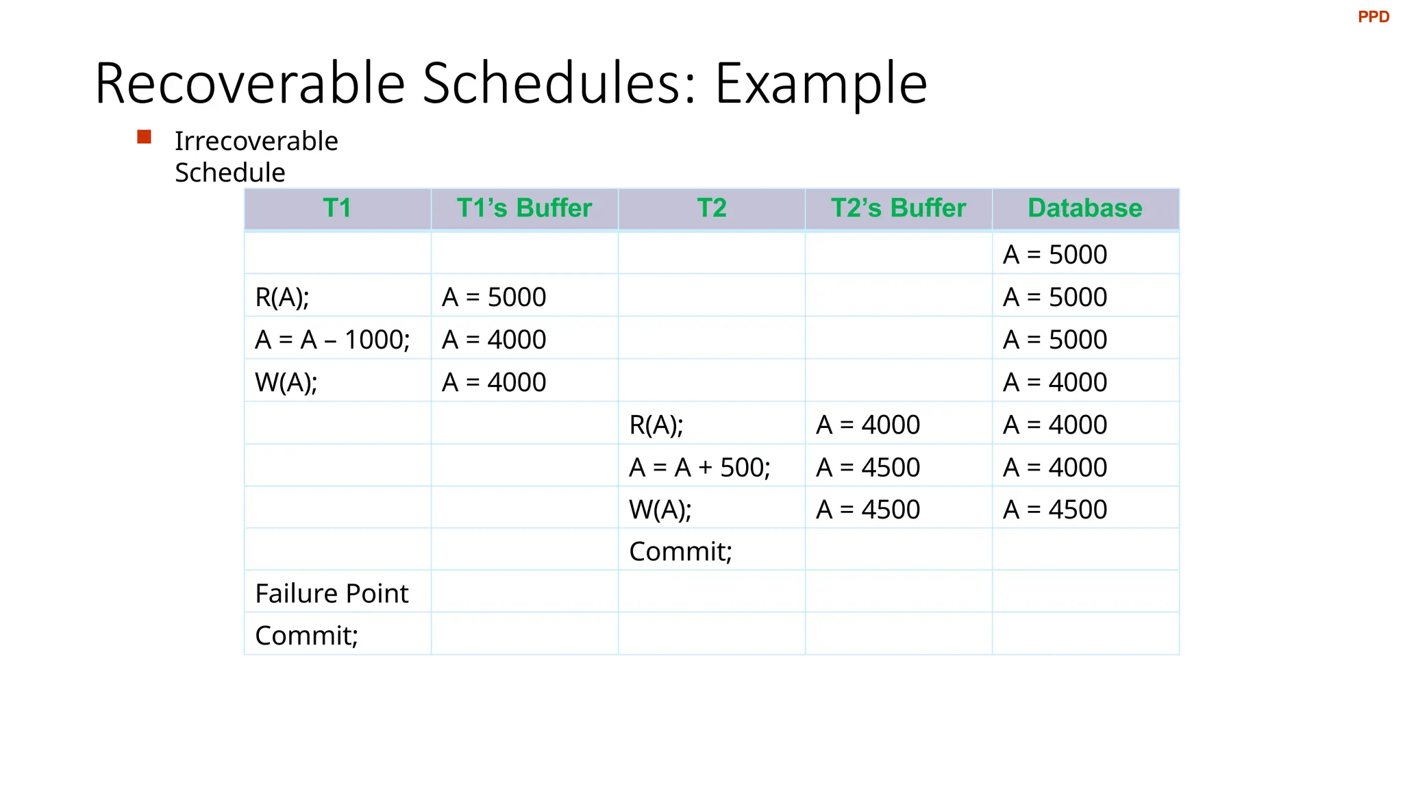
Recoverable Schedules: Example
 Irrecoverable
Schedule
T1 T1’s Buffer T2 T2’s Buffer Database
A = 5000
R(A); A = 5000 A = 5000
A = A – 1000; A = 4000 A = 5000
W(A); A = 4000 A = 4000
R(A); A = 4000 A = 4000
A = A + 500; A = 4500 A = 4000
W(A); A = 4500 A = 4500
Commit;
Failure Point
Commit;
PPD

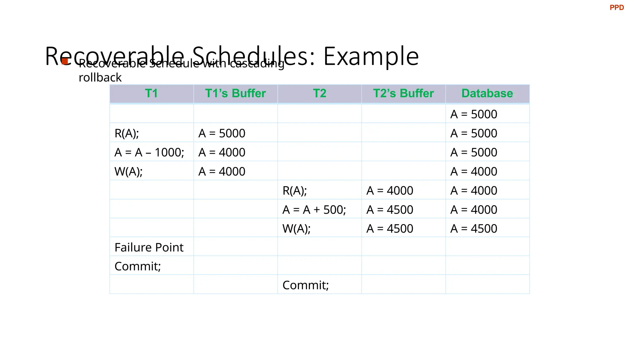
 Recoverable Schedule with cascading
rollback
A = 5000
R(A); A = 5000 A = 5000
A = A – 1000; A = 4000 A = 5000
W(A); A = 4000 A = 4000
R(A); A = 4000 A = 4000
A = A + 500; A = 4500 A = 4000
W(A); A = 4500 A = 4500
Failure Point
Commit;
Commit;
PPD

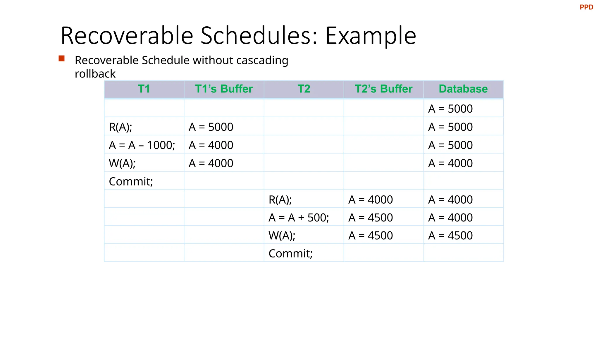
 Recoverable Schedule without cascading
rollback
A = 5000
R(A); A = 5000 A = 5000
A = A – 1000; A = 4000 A = 5000
W(A); A = 4000 A = 4000
Commit;
R(A); A = 4000 A = 4000
A = A + 500; A = 4500 A = 4000
W(A); A = 4500 A = 4500
Commit;
PPD

RECOVERY AND ATOMICITY
PPD
• Failure Classification
• Storage Structure
• Recovery and
Atomicity
• Log-
Based
Recovery

Recovery and Atomicity
 To ensure atomicity despite failures, we first output information describing the
modifications to stable storage without modifying the database itself
 We study log-based recovery mechanisms in detail
 We first present key concepts
 And then present the actual recovery algorithm
 Less used alternative: shadow-paging
 In this Module we assume serial execution of transactions
 In the next Module, we consider the case of concurrent transaction execution

LOG-BASED RECOVERY
• Failure Classification
• Storage Structure
• Recovery
and
Atomicity
• Log-Based
Recovery

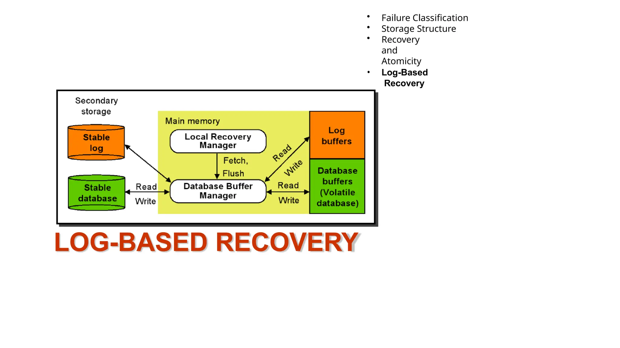
Log-Based Recovery
 A log is kept on stable storage
 The log is a sequence of log records, which maintains information about update
activities on the database
 When transaction Ti starts, it registers itself by writing a record
<Ti start>
to the log
 Before Ti executes write(X), a log record
<Ti, X, V1, V2>
is written, where V1 is the value of X before the write (the old value), and V2 is the value
to be written to X (the new value)
 When Ti finishes it last statement, the log record <Ti commit> is written
 Two approaches using logs
 Immediate database modification
 Deferred database modification

Database Modification
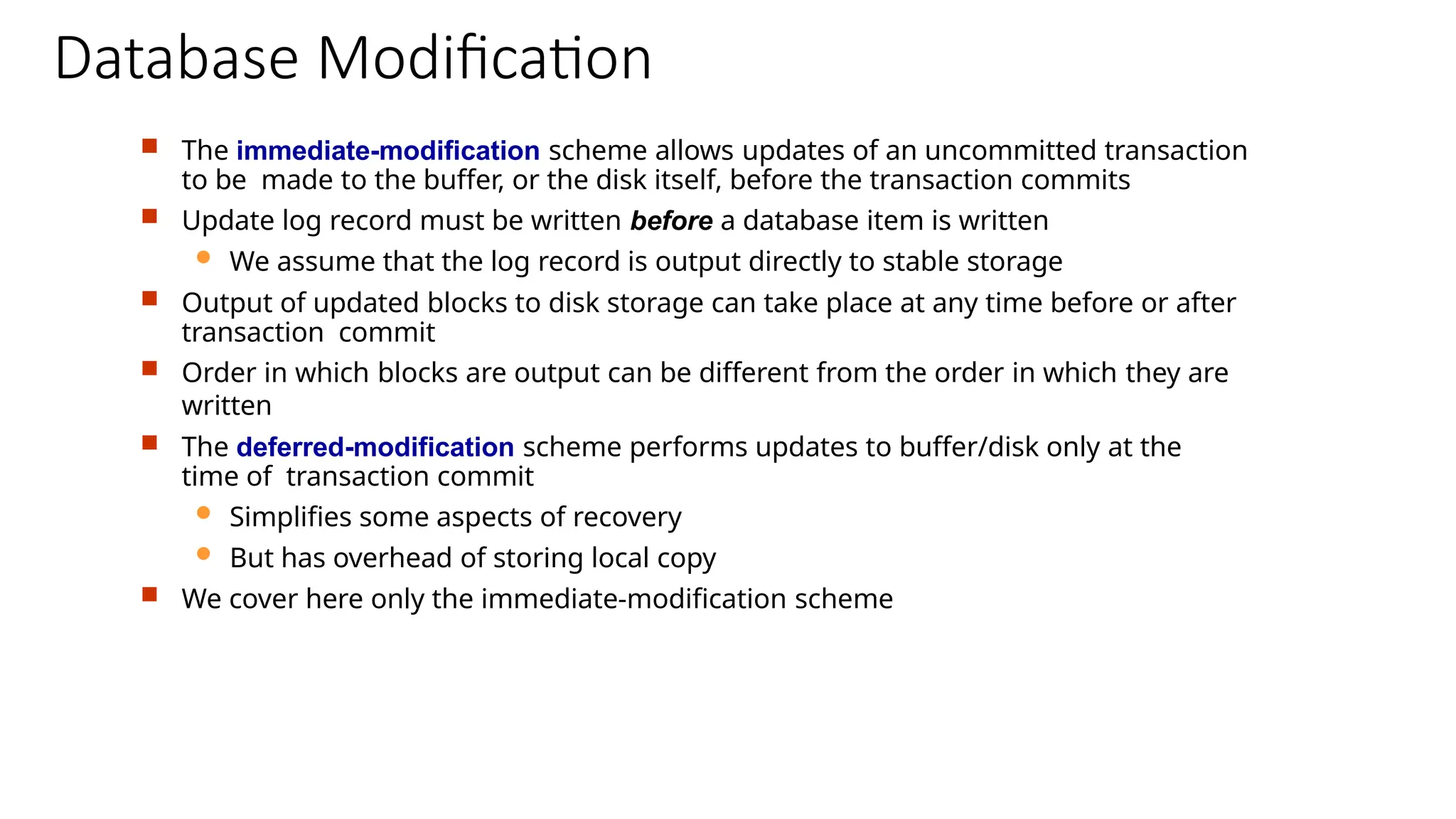
 The immediate-modification scheme allows updates of an uncommitted transaction
to be made to the buffer, or the disk itself, before the transaction commits
 Update log record must be written before a database item is written
 We assume that the log record is output directly to stable storage
 Output of updated blocks to disk storage can take place at any time before or after
transaction commit
 Order in which blocks are output can be different from the order in which they are
written
 The deferred-modification scheme performs updates to buffer/disk only at the
time of transaction commit
 Simplifies some aspects of recovery
 But has overhead of storing local copy
 We cover here only the immediate-modification scheme

Transaction Commit
 A transaction is said to have committed when its commit log record is output to stable
storage
 All previous log records of the transaction must have been output already
 Writes performed by a transaction may still be in the buffer when the transaction
commits, and may be output later

Immediate Database Modification Example
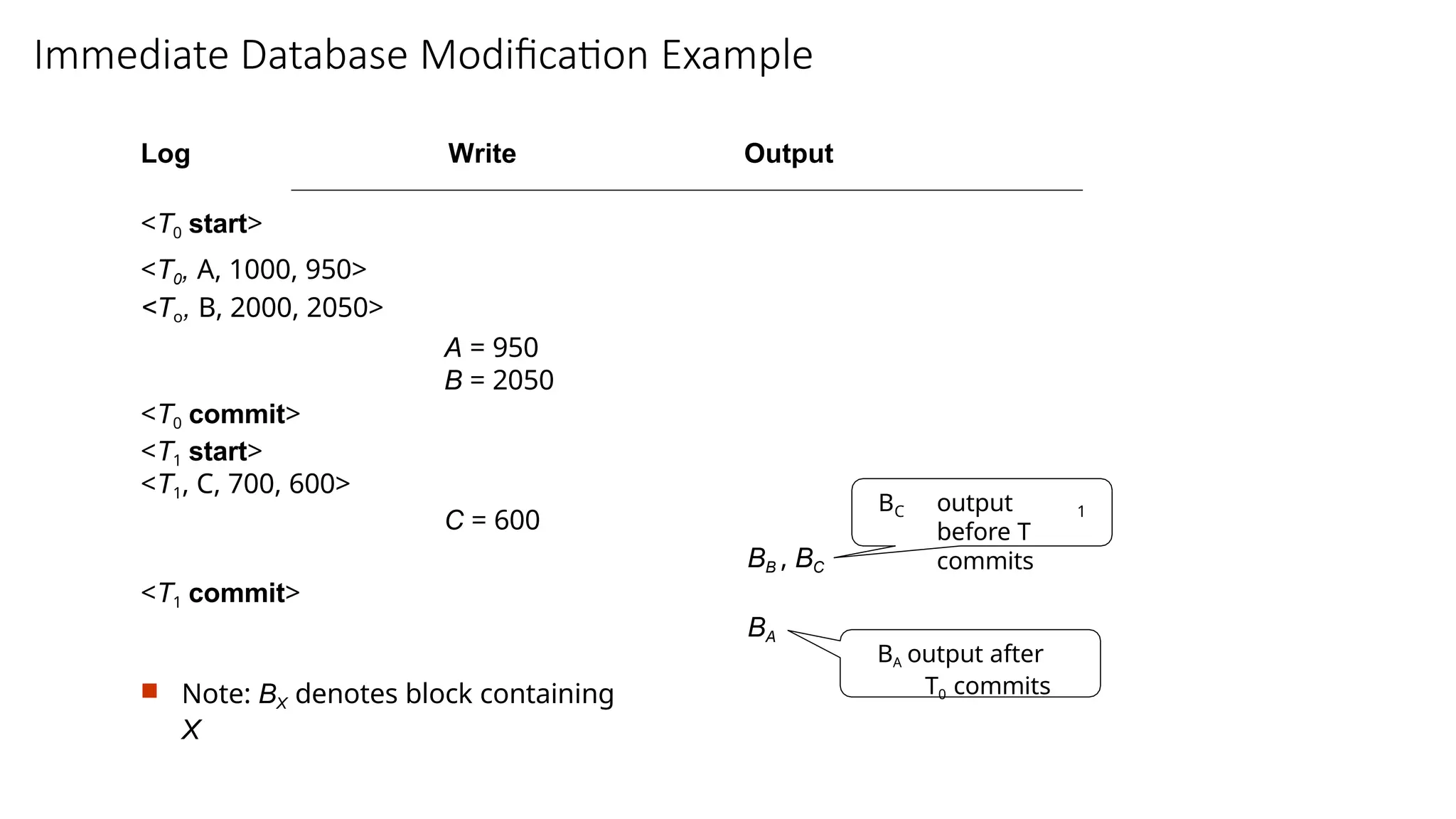
Log Write Output
<T0 start>
<T0, A, 1000, 950>
<To, B, 2000, 2050>
A = 950
B = 2050
<T0 commit>
<T1 start>
<T1, C, 700, 600>
C = 600
BB , BC
<T1 commit>
BA
 Note: BX denotes block containing
X
C 1
B output
before T
commits
BA output after
T0 commits

Undo and Redo Operations
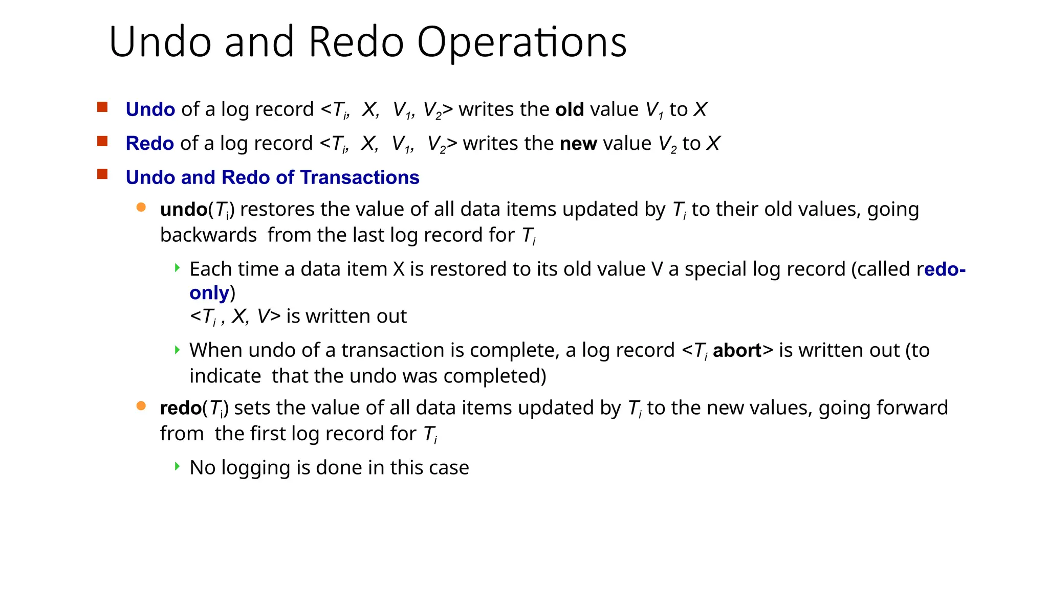
 Undo of a log record <Ti, X, V1, V2> writes the old value V1 to X
 Redo of a log record <Ti, X, V1, V2> writes the new value V2 to X
 Undo and Redo of Transactions
 undo(Ti) restores the value of all data items updated by Ti to their old values, going
backwards from the last log record for Ti
 Each time a data item X is restored to its old value V a special log record (called redo-
only)
<Ti , X, V> is written out
 When undo of a transaction is complete, a log record <Ti abort> is written out (to
indicate that the undo was completed)
 redo(Ti) sets the value of all data items updated by Ti to the new values, going forward
from the first log record for Ti
 No logging is done in this case

Undo and Redo Operations (Cont.)
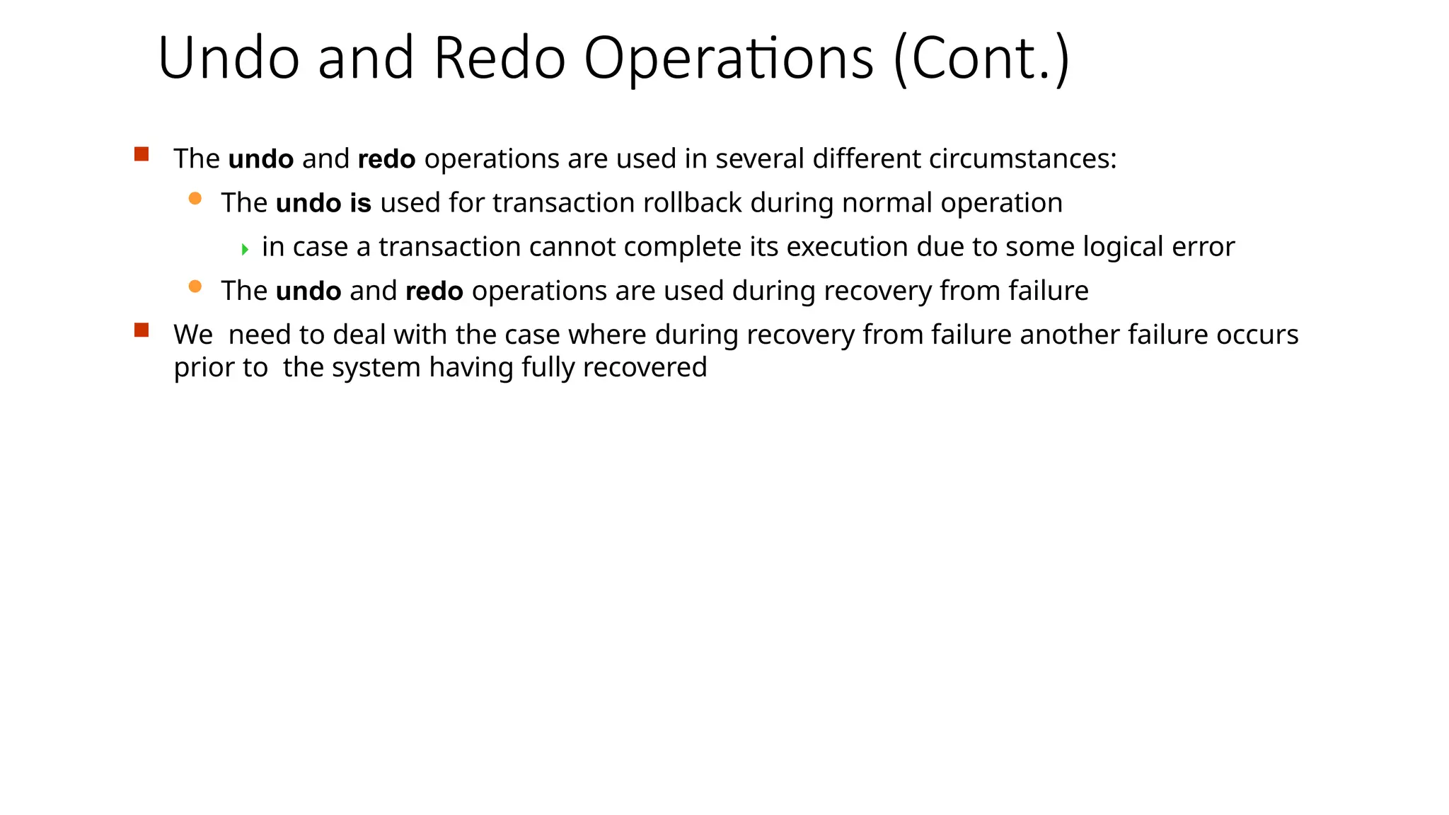
 The undo and redo operations are used in several different circumstances:
 The undo is used for transaction rollback during normal operation
 in case a transaction cannot complete its execution due to some logical error
 The undo and redo operations are used during recovery from failure
 We need to deal with the case where during recovery from failure another failure occurs
prior to the system having fully recovered

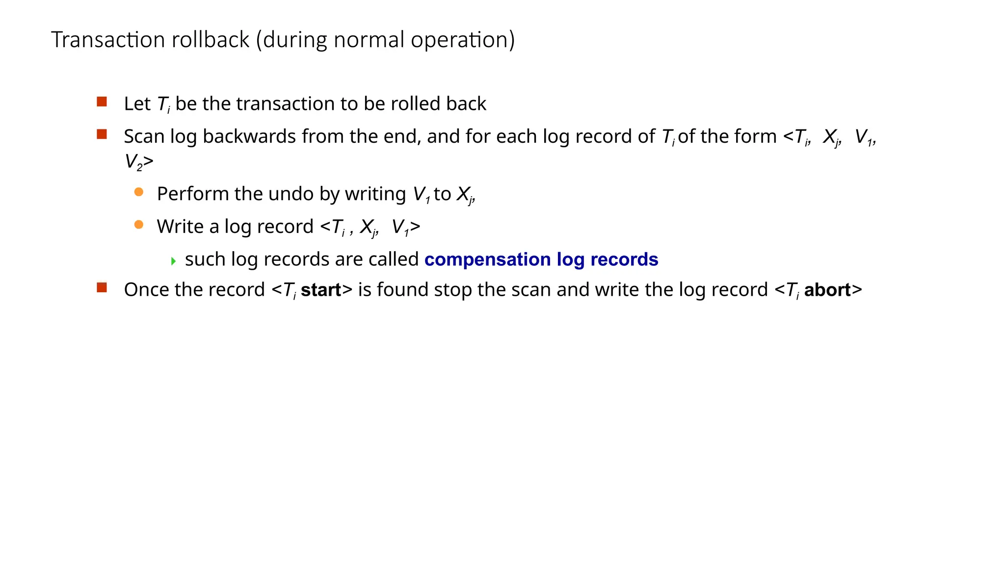
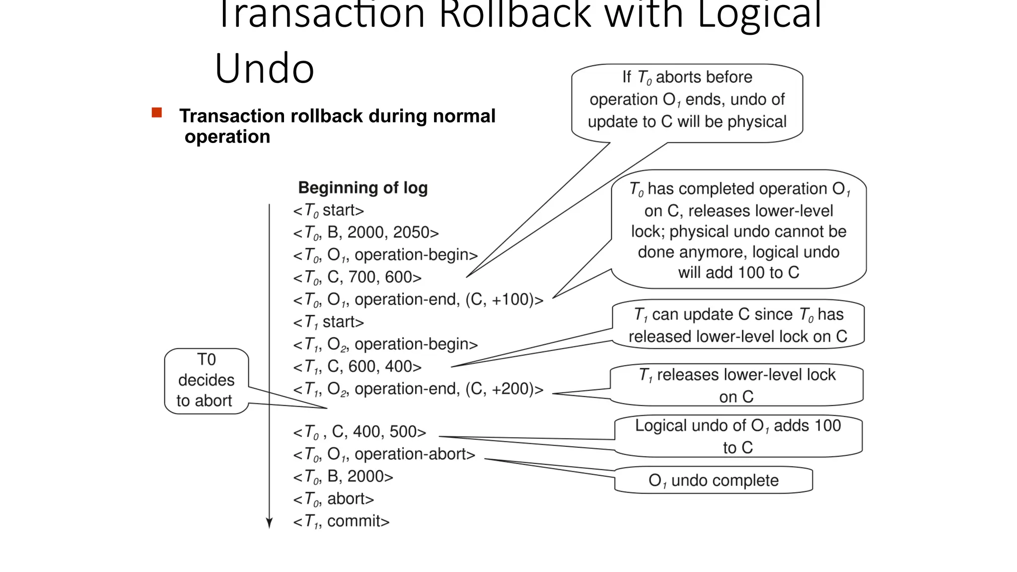
Transaction rollback (during normal operation)
 Let Ti be the transaction to be rolled back
 Scan log backwards from the end, and for each log record of Ti of the form <Ti, Xj, V1,
V2>
 Perform the undo by writing V1 to Xj,
 Write a log record <Ti , Xj, V1>
 such log records are called compensation log records
 Once the record <Ti start> is found stop the scan and write the log record <Ti abort>

Undo and Redo on Recovering from Failure
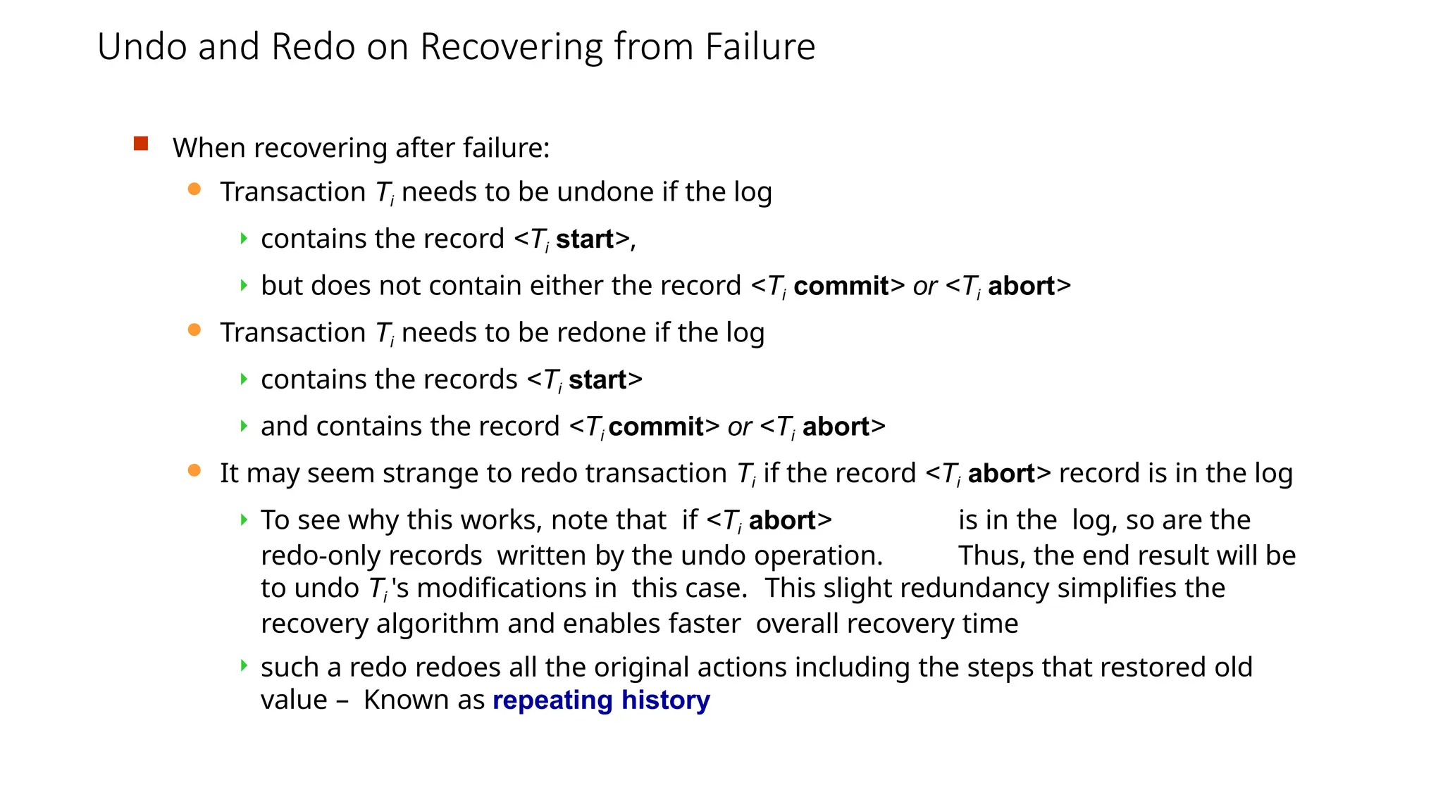
 When recovering after failure:
 Transaction Ti needs to be undone if the log
 contains the record <Ti start>,
 but does not contain either the record <Ti commit> or <Ti abort>
 Transaction Ti needs to be redone if the log
 contains the records <Ti start>
 and contains the record <Ti commit> or <Ti abort>
 It may seem strange to redo transaction Ti if the record <Ti abort> record is in the log
 To see why this works, note that if <Ti abort> is in the log, so are the
redo-only records written by the undo operation. Thus, the end result will be
to undo Ti 's modifications in this case. This slight redundancy simplifies the
recovery algorithm and enables faster overall recovery time
 such a redo redoes all the original actions including the steps that restored old
value – Known as repeating history

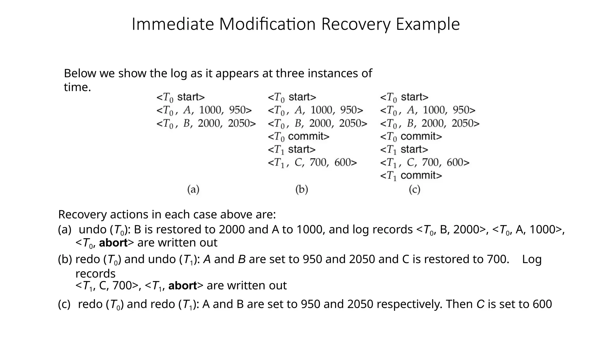
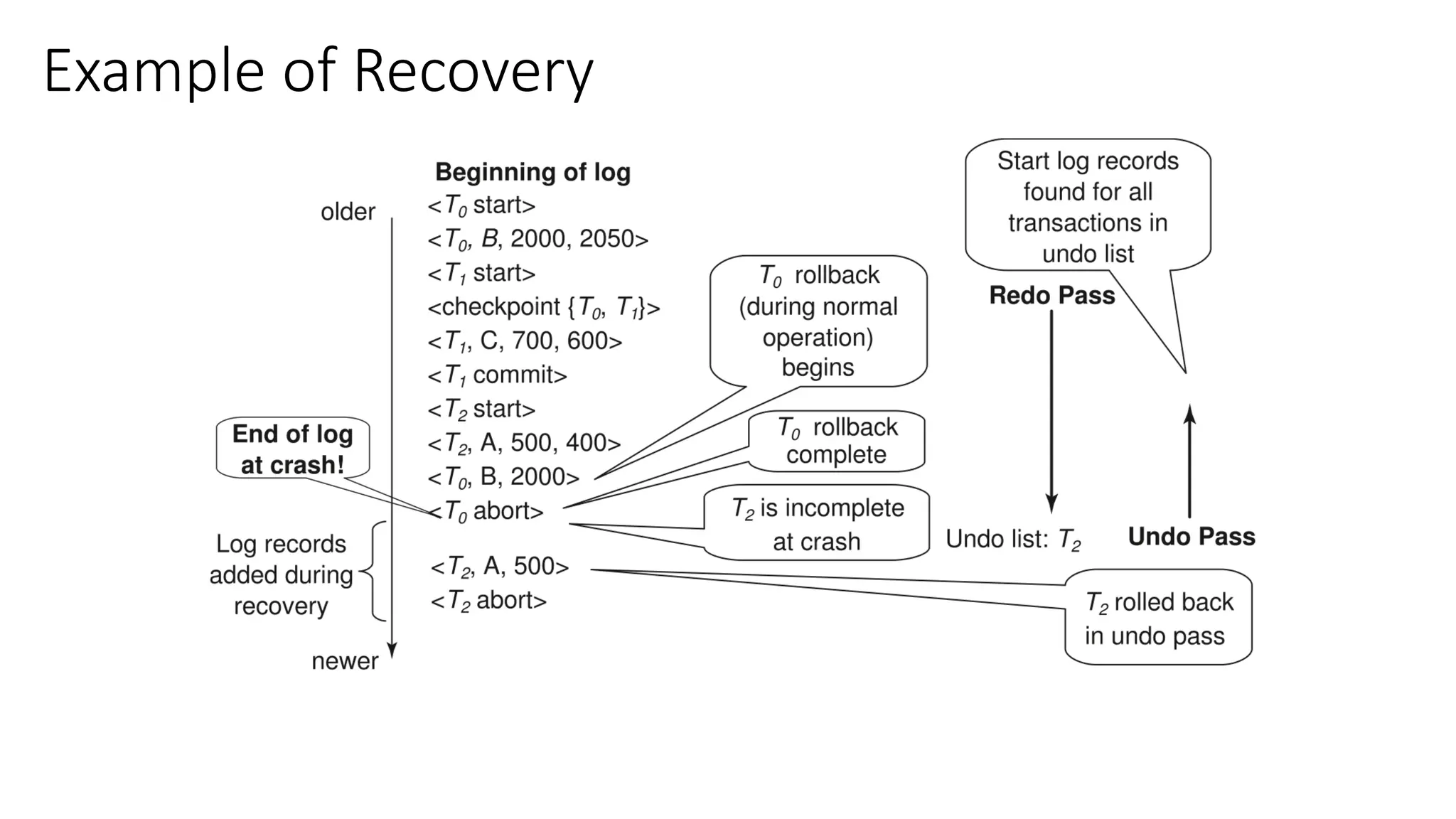
Immediate Modification Recovery Example
Below we show the log as it appears at three instances of
time.
Recovery actions in each case above are:
(a) undo (T0): B is restored to 2000 and A to 1000, and log records <T0, B, 2000>, <T0, A, 1000>,
<T0, abort> are written out
(b) redo (T0) and undo (T1): A and B are set to 950 and 2050 and C is restored to 700. Log
records
<T1, C, 700>, <T1, abort> are written out
(c) redo (T0) and redo (T1): A and B are set to 950 and 2050 respectively. Then C is set to 600

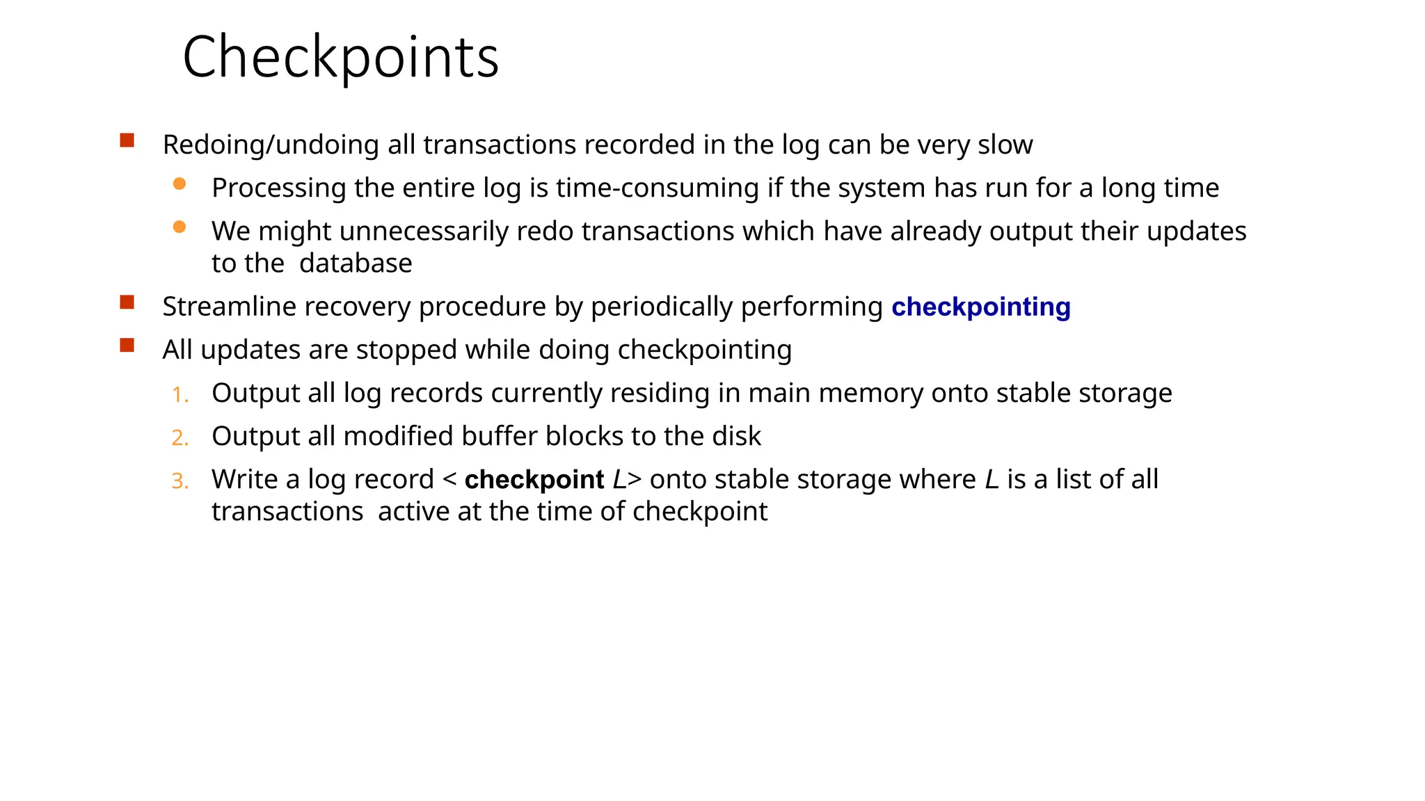
Checkpoints
 Redoing/undoing all transactions recorded in the log can be very slow
 Processing the entire log is time-consuming if the system has run for a long time
 We might unnecessarily redo transactions which have already output their updates
to the database
 Streamline recovery procedure by periodically performing checkpointing
 All updates are stopped while doing checkpointing
1. Output all log records currently residing in main memory onto stable storage
2. Output all modified buffer blocks to the disk
3. Write a log record < checkpoint L> onto stable storage where L is a list of all
transactions active at the time of checkpoint

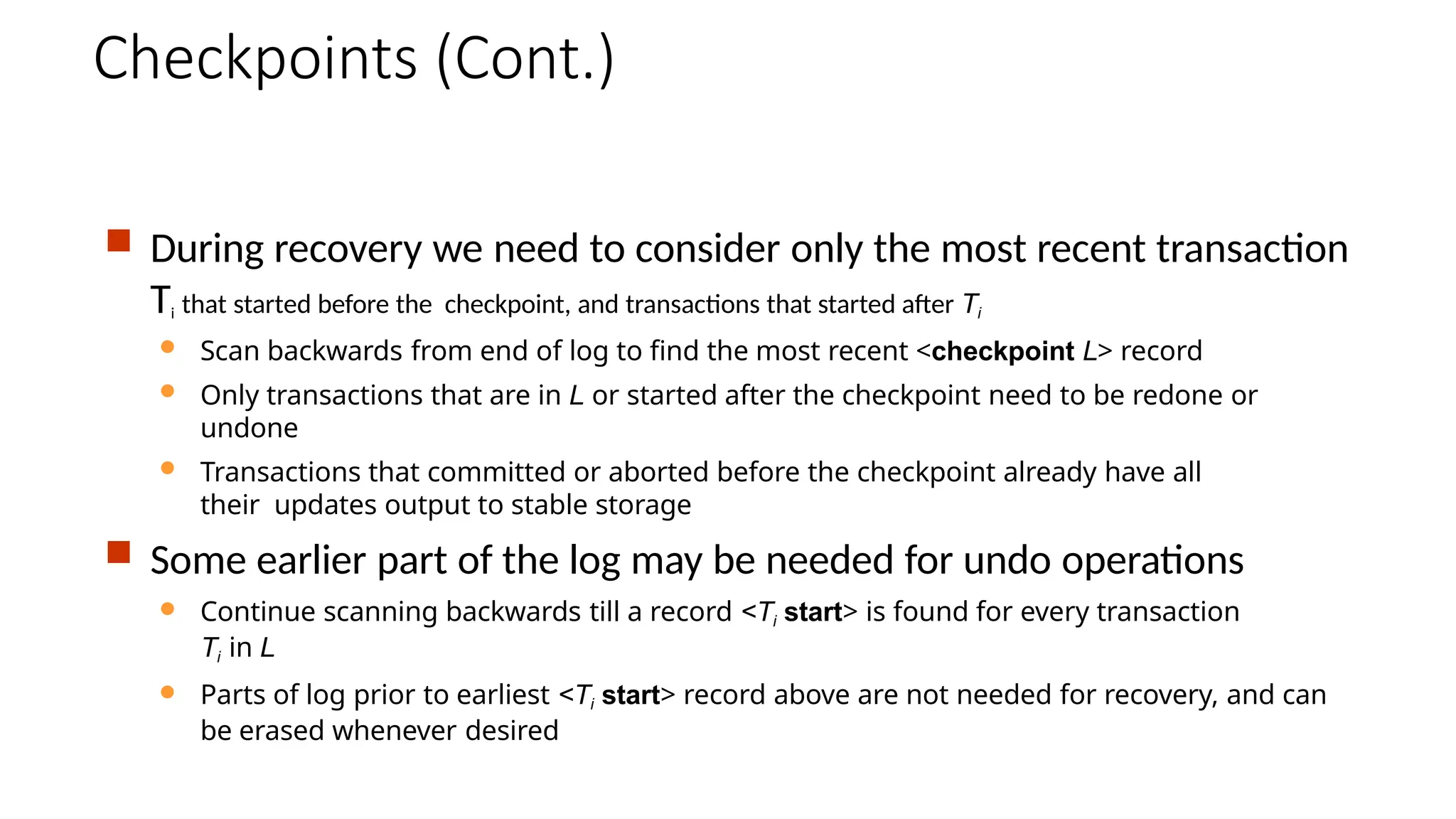
Checkpoints (Cont.)
 During recovery we need to consider only the most recent transaction
Ti that started before the checkpoint, and transactions that started after Ti
 Scan backwards from end of log to find the most recent <checkpoint L> record
 Only transactions that are in L or started after the checkpoint need to be redone or
undone
 Transactions that committed or aborted before the checkpoint already have all
their updates output to stable storage
 Some earlier part of the log may be needed for undo operations
 Continue scanning backwards till a record <Ti start> is found for every transaction
Ti in L
 Parts of log prior to earliest <Ti start> record above are not needed for recovery, and can
be erased whenever desired

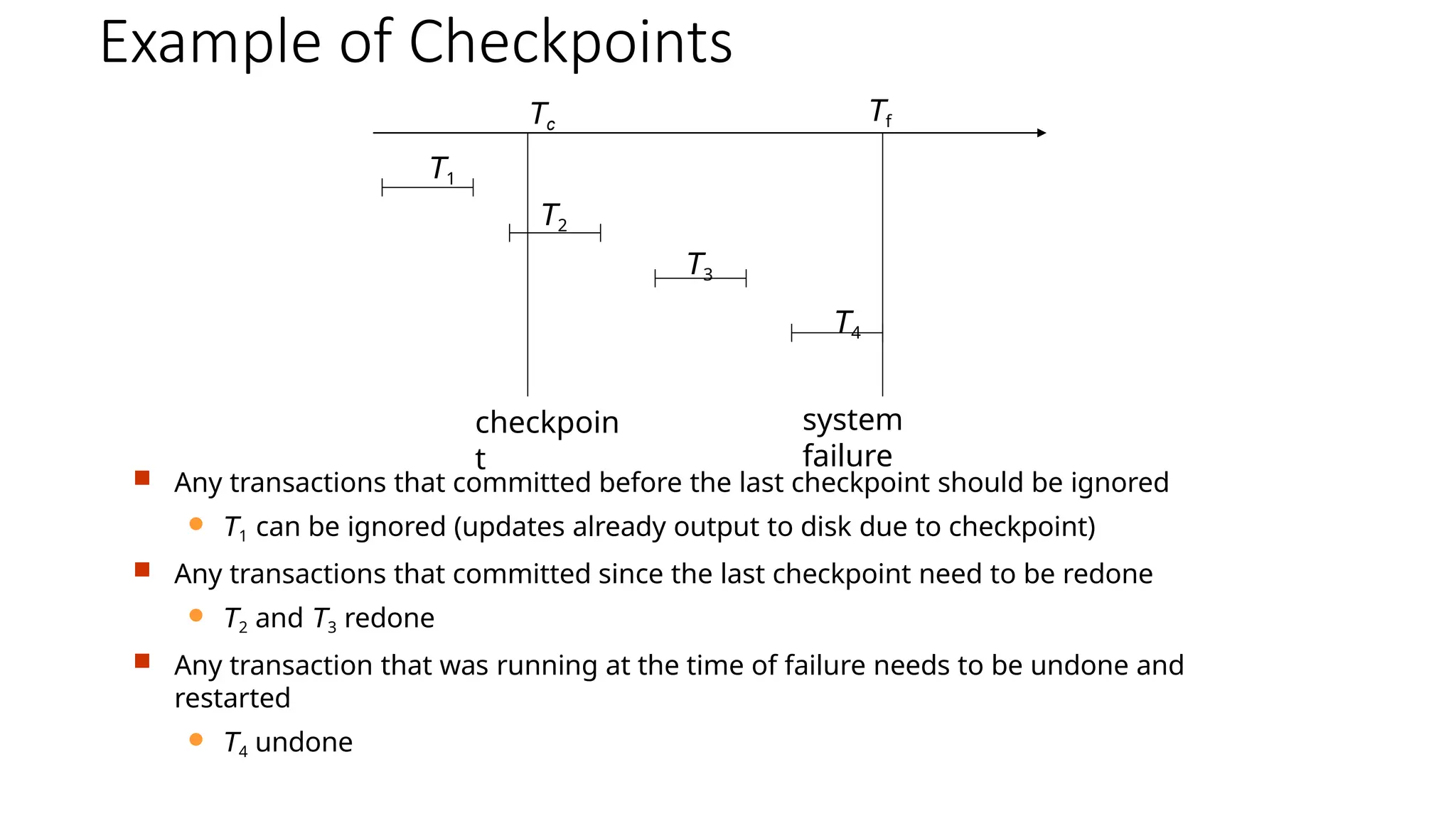
Example of Checkpoints
 Any transactions that committed before the last checkpoint should be ignored
 T1 can be ignored (updates already output to disk due to checkpoint)
 Any transactions that committed since the last checkpoint need to be redone
 T2 and T3 redone
 Any transaction that was running at the time of failure needs to be undone and
restarted
 T4 undone
Tc
Tf
T1
T2
T3
T4
checkpoin
t
system
failure

RECOVERY ALGORITHM
• Recovery
Algorithm
• Recovery with
Early Lock Release

Recovery Schemes
 So far:
 We covered key concepts
 We assumed serial execution of transactions
 Now:
 We discuss concurrency control issues
 We present the components of the basic recovery
algorithm

Concurrency Control and Recovery
 With concurrent transactions, all transactions share a single disk buffer and a single log
 A buffer block can have data items updated by one or more transactions
 We assume that if a transaction Ti has modified an item, no other transaction can modify
the same item until Ti has committed or aborted
 That is, the updates of uncommitted transactions should not be visible to other
transactions
 Otherwise how do we perform undo if T1 updates A, then T2 updates A and
commits, and finally T1 has to abort?
 Can be ensured by obtaining exclusive locks on updated items and holding the locks
till end of transaction (strict two-phase locking)
 Log records of different transactions may be interspersed in the log

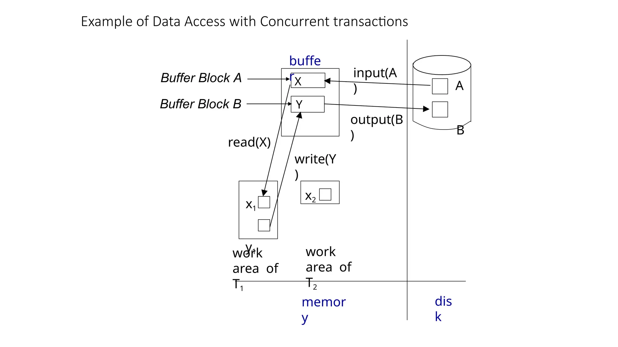
Example of Data Access with Concurrent transactions
X
Y
A
B
x1
y1
buffe
r
Buffer Block A
Buffer Block B
input(A
)
output(B
)
read(X)
write(Y
)
dis
k
work
area of
T1
work
area of
T2
memor
y
x2

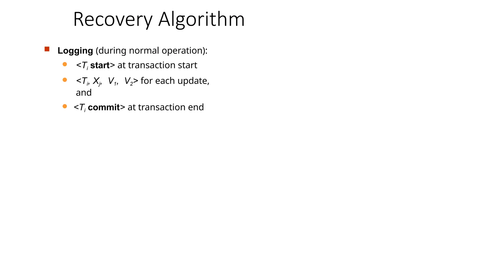
Recovery Algorithm
 Logging (during normal operation):
 <Ti start> at transaction start
 <Ti, Xj, V1, V2> for each update,
and
 <Ti commit> at transaction end

Recovery Algorithm
(Contd.)
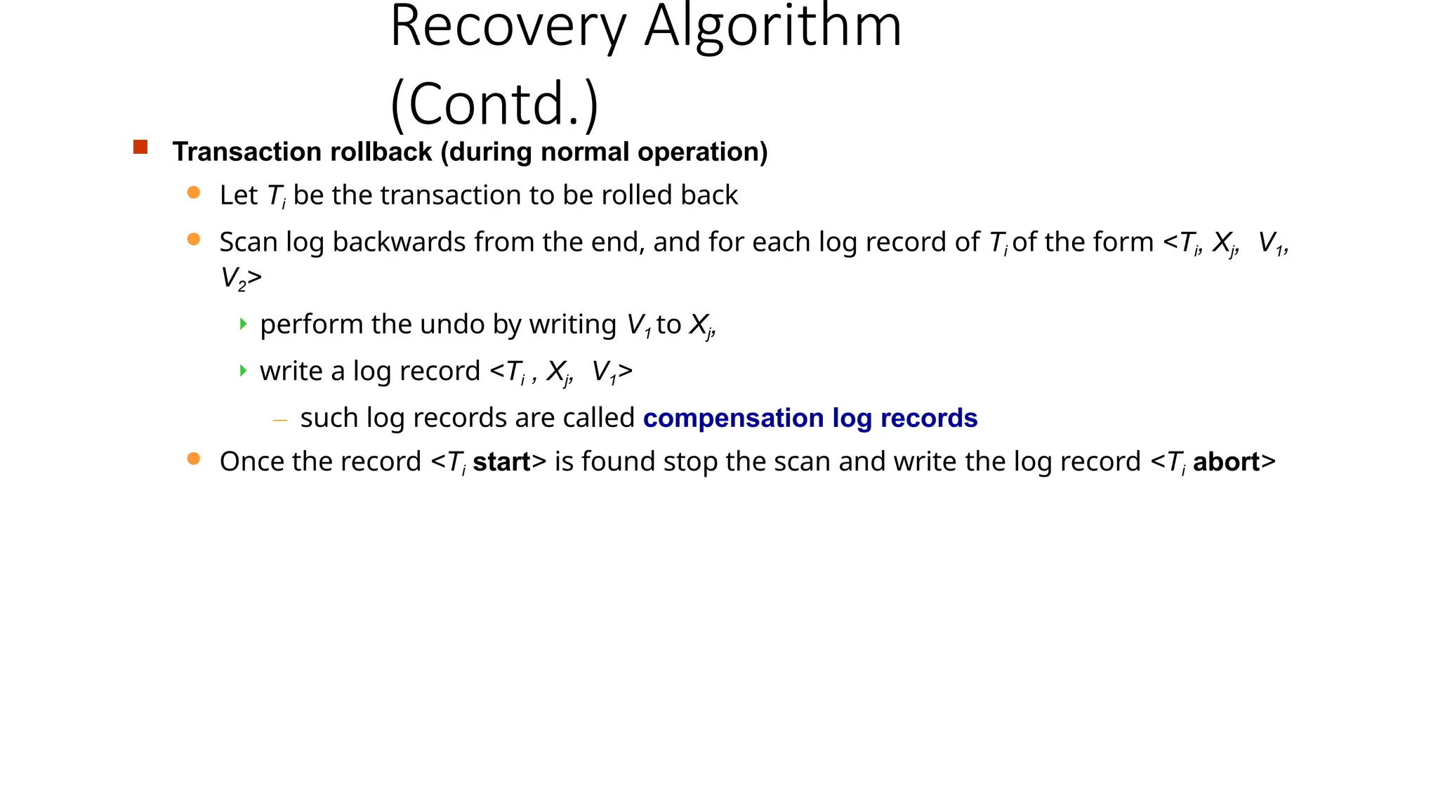
 Transaction rollback (during normal operation)
 Let Ti be the transaction to be rolled back
 Scan log backwards from the end, and for each log record of Ti of the form <Ti, Xj, V1,
V2>
 perform the undo by writing V1 to Xj,
 write a log record <Ti , Xj, V1>
– such log records are called compensation log records
 Once the record <Ti start> is found stop the scan and write the log record <Ti abort>

Recovery Algorithm (Cont.)
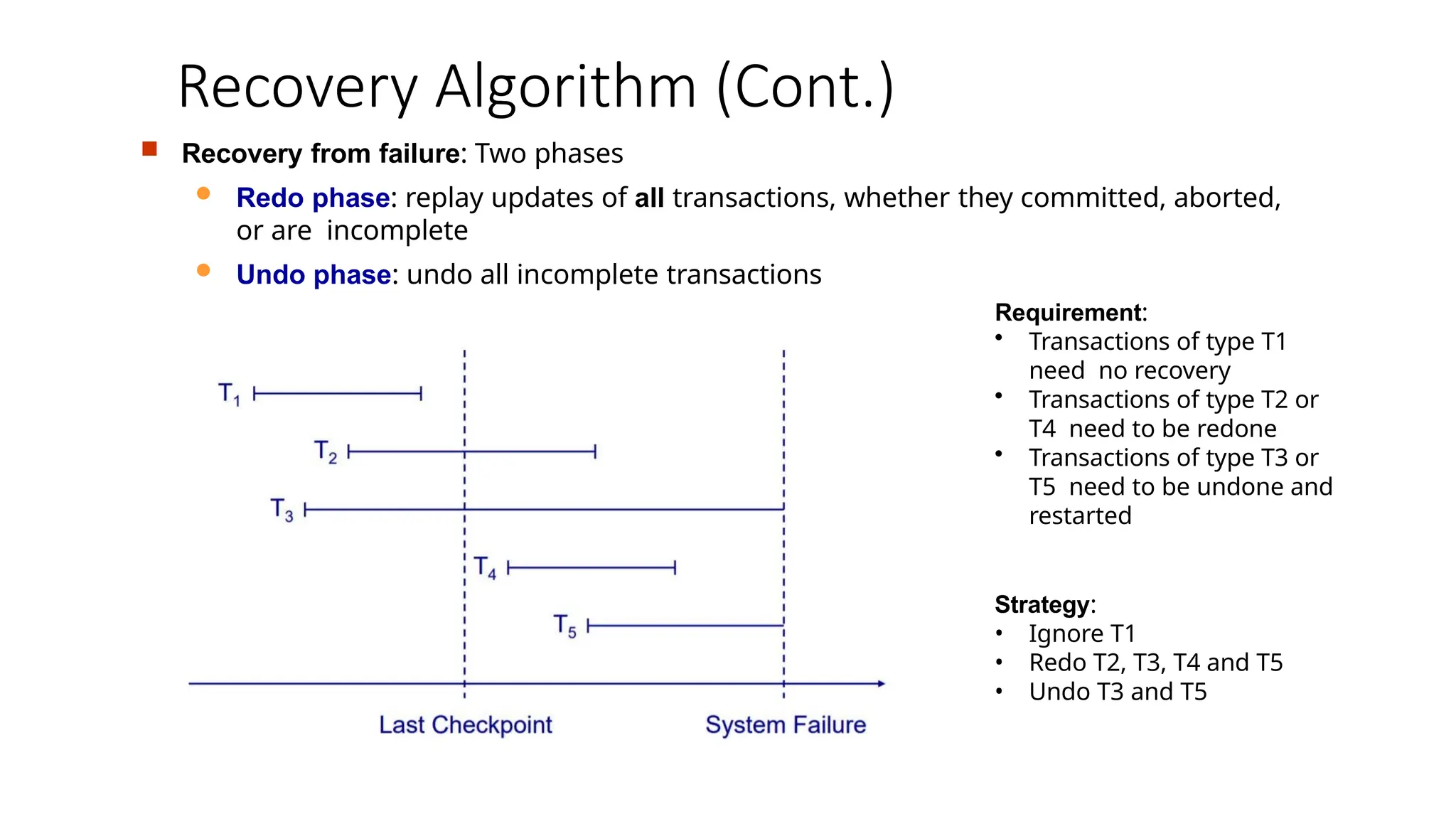
 Recovery from failure: Two phases
 Redo phase: replay updates of all transactions, whether they committed, aborted,
or are incomplete
 Undo phase: undo all incomplete transactions
Requirement:
• Transactions of type T1
need no recovery
• Transactions of type T2 or
T4 need to be redone
• Transactions of type T3 or
T5 need to be undone and
restarted
Strategy:
• Ignore T1
• Redo T2, T3, T4 and T5
• Undo T3 and T5

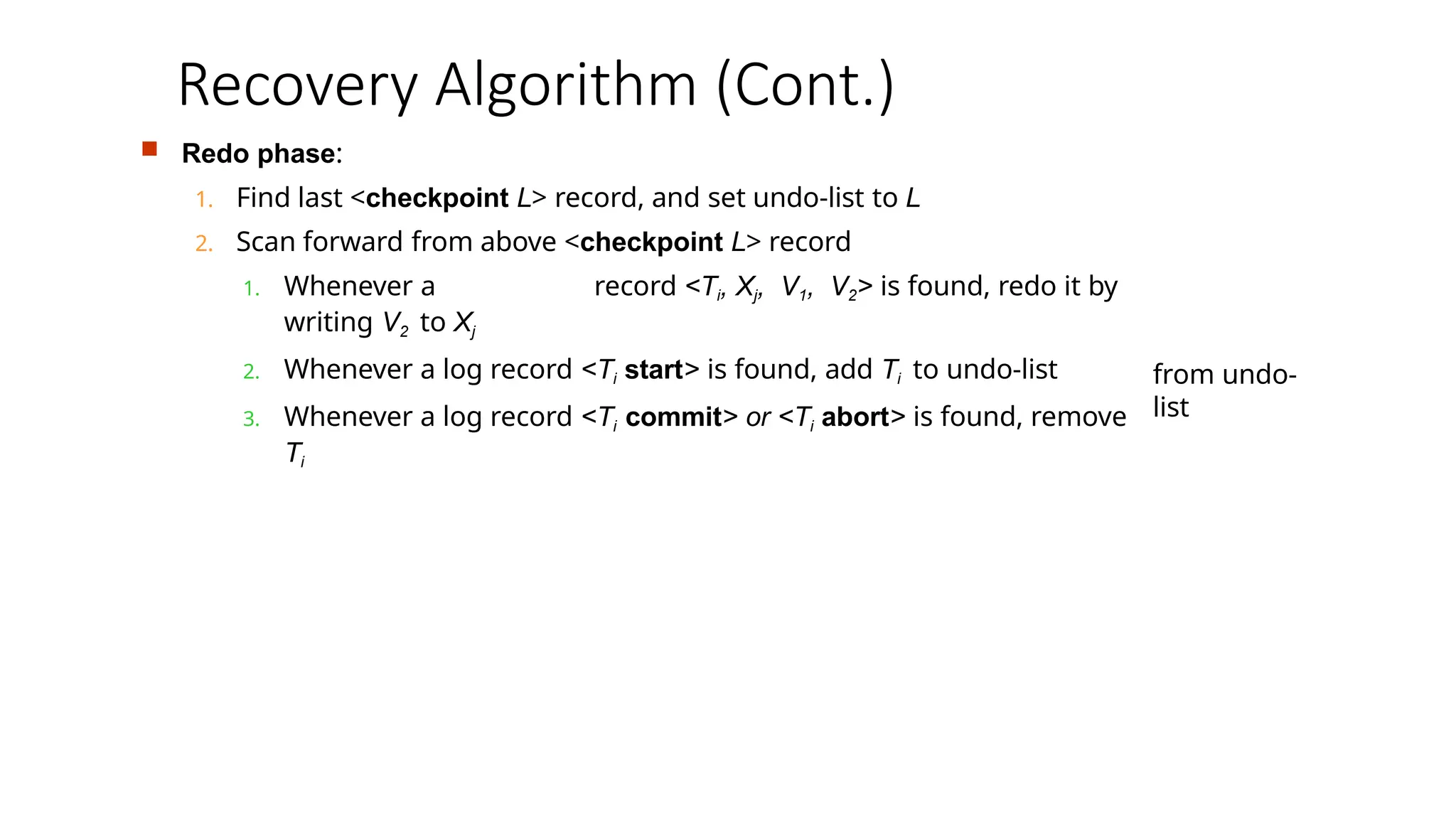
 Redo phase:
1. Find last <checkpoint L> record, and set undo-list to L
2. Scan forward from above <checkpoint L> record
1. Whenever a record <Ti, Xj, V1, V2> is found, redo it by
writing V2 to Xj
2. Whenever a log record <Ti start> is found, add Ti to undo-list
3. Whenever a log record <Ti commit> or <Ti abort> is found, remove
Ti
from undo-
list

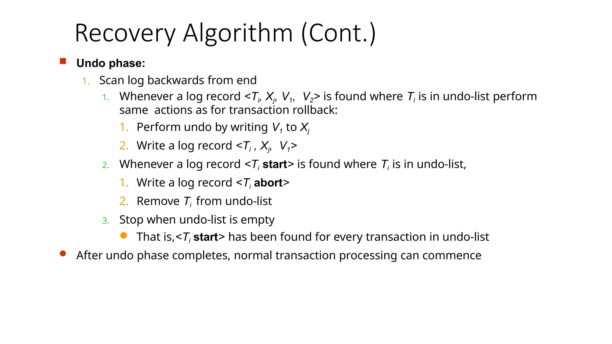
 Undo phase:
1. Scan log backwards from end
1. Whenever a log record <Ti, Xj, V1, V2> is found where Ti is in undo-list perform
same actions as for transaction rollback:
1. Perform undo by writing V1 to Xj
2. Write a log record <Ti , Xj, V1>
2. Whenever a log record <Ti start> is found where Ti is in undo-list,
1. Write a log record <Ti abort>
2. Remove Ti from undo-list
3. Stop when undo-list is empty
 That is,<Ti start> has been found for every transaction in undo-list
 After undo phase completes, normal transaction processing can commence

RECOVERY WITH EARLY LOCK
RELEASE
• Recovery
Algorithm
• Recovery with
Early Lock Release

Recovery with Early Lock Release
 Support for high-concurrency locking techniques, such as those used for B+-tree
concurrency control, which release locks early
 Supports “logical undo”
 Recovery based on “repeating history”, whereby recovery executes exactly the same
actions as normal processing

Logical Undo Logging
 Operations like B+-tree insertions and deletions release locks early
 They cannot be undone by restoring old values (physical undo), since once a
lock is released, other transactions may have updated the B+-tree
 Instead, insertions (resp. deletions) are undone by executing a deletion (resp.
insertion) operation (known as logical undo)
 For such operations, undo log records should contain the undo operation to be
executed
 Such logging is called logical undo logging, in contrast to physical undo logging
 Operations are called logical operations
 Other examples:
 delete of tuple, to undo insert of tuple
– allows early lock release on space allocation information
 subtract amount deposited, to undo deposit
– allows early lock release on bank balance

Physical Redo
 Redo information is logged physically (that is, new value for each write) even for
operations with logical undo
 Logical redo is very complicated since database state on disk may not be
“operation consistent” when recovery starts
 Physical redo logging does not conflict with early lock release

Operation Logging
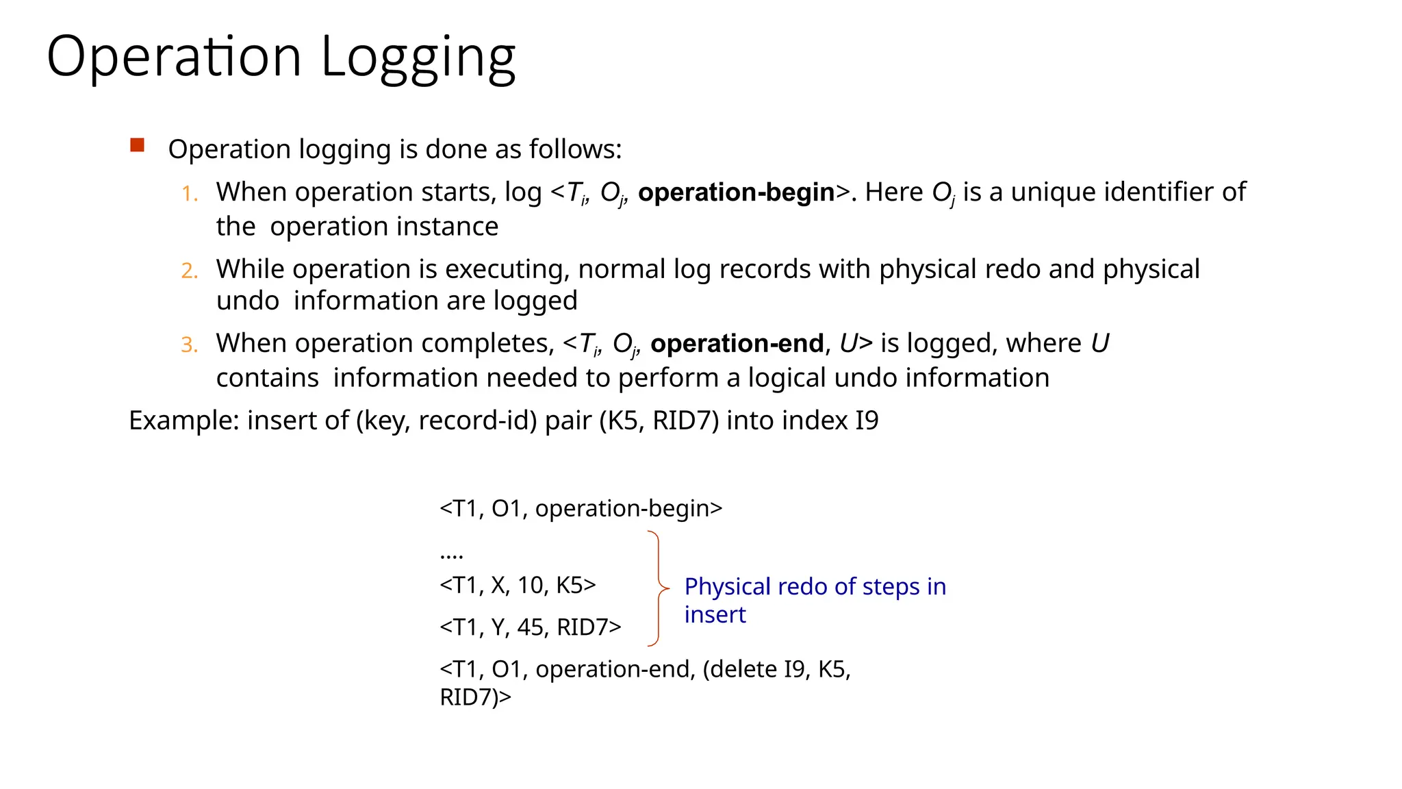
 Operation logging is done as follows:
1. When operation starts, log <Ti, Oj, operation-begin>. Here Oj is a unique identifier of
the operation instance
2. While operation is executing, normal log records with physical redo and physical
undo information are logged
3. When operation completes, <Ti, Oj, operation-end, U> is logged, where U
contains information needed to perform a logical undo information
Example: insert of (key, record-id) pair (K5, RID7) into index I9
<T1, O1, operation-begin>
….
<T1, X, 10, K5>
<T1, Y, 45, RID7>
<T1, O1, operation-end, (delete I9, K5,
RID7)>
Physical redo of steps in
insert

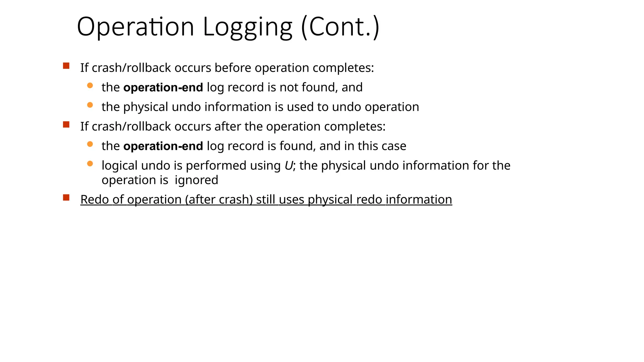
Operation Logging (Cont.)
 If crash/rollback occurs before operation completes:
 the operation-end log record is not found, and
 the physical undo information is used to undo operation
 If crash/rollback occurs after the operation completes:
 the operation-end log record is found, and in this case
 logical undo is performed using U; the physical undo information for the
operation is ignored
 Redo of operation (after crash) still uses physical redo information

Transaction Rollback with Logical Undo
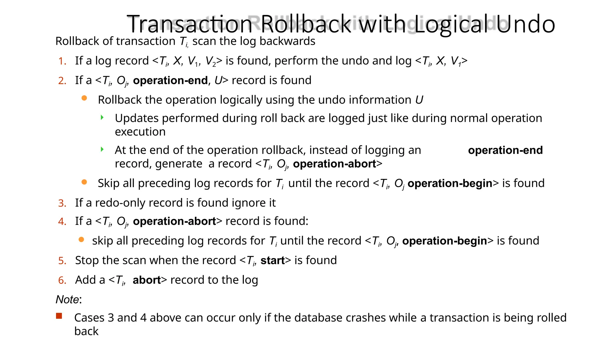
Rollback of transaction Ti, scan the log backwards
1. If a log record <Ti, X, V1, V2> is found, perform the undo and log <Ti, X, V1>
2. If a <Ti, Oj, operation-end, U> record is found
 Rollback the operation logically using the undo information U
 Updates performed during roll back are logged just like during normal operation
execution
 At the end of the operation rollback, instead of logging an operation-end
record, generate a record <Ti, Oj, operation-abort>
 Skip all preceding log records for Ti until the record <Ti, Oj operation-begin> is found
3. If a redo-only record is found ignore it
4. If a <Ti, Oj, operation-abort> record is found:
 skip all preceding log records for Ti until the record <Ti, Oj, operation-begin> is found
5. Stop the scan when the record <Ti, start> is found
6. Add a <Ti, abort> record to the log
Note:
 Cases 3 and 4 above can occur only if the database crashes while a transaction is being rolled
back

Transaction Rollback with Logical
Undo
 Transaction rollback during normal
operation

Failure Recovery with Logical
Undo

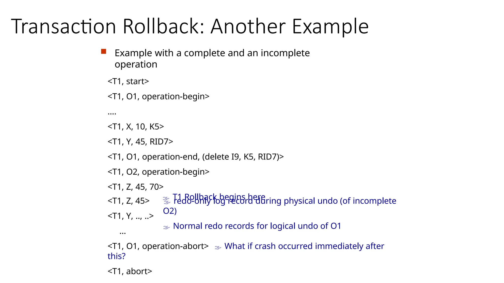
Transaction Rollback: Another Example
 Example with a complete and an incomplete
operation
<T1, start>
….
<T1, X, 10, K5>
<T1, Y, 45, RID7>
<T1, O1, operation-end, (delete I9, K5, RID7)>
<T1, Z, 45, 70>
 T1 Rollback begins here
 redo-only log record during physical undo (of incomplete
O2)
 Normal redo records for logical undo of O1
<T1, Z, 45>
<T1, Y, .., ..>
…
<T1, O1, operation-abort>  What if crash occurred immediately after
this?
<T1, abort>

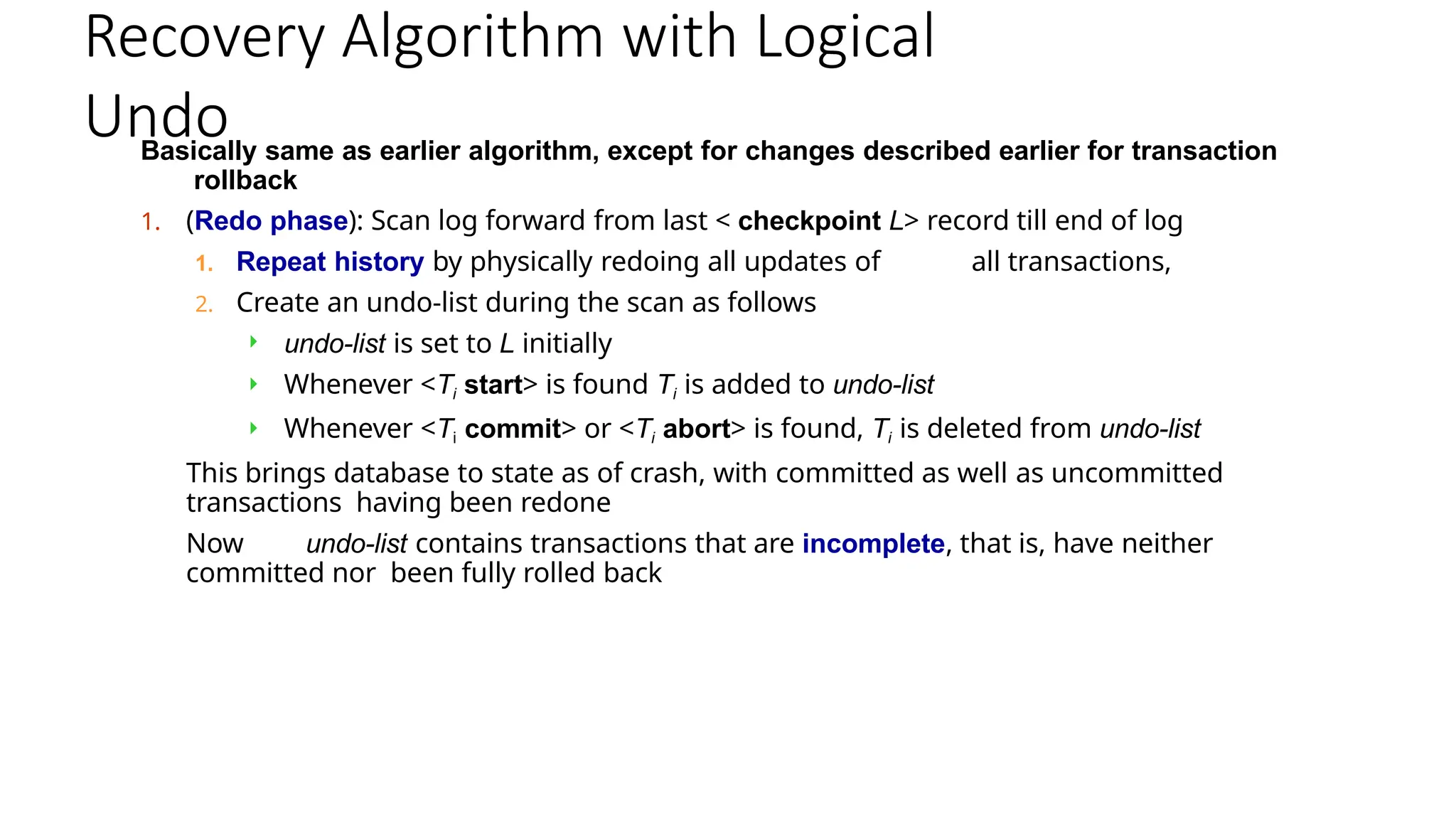
Recovery Algorithm with Logical
Undo
Basically same as earlier algorithm, except for changes described earlier for transaction
rollback
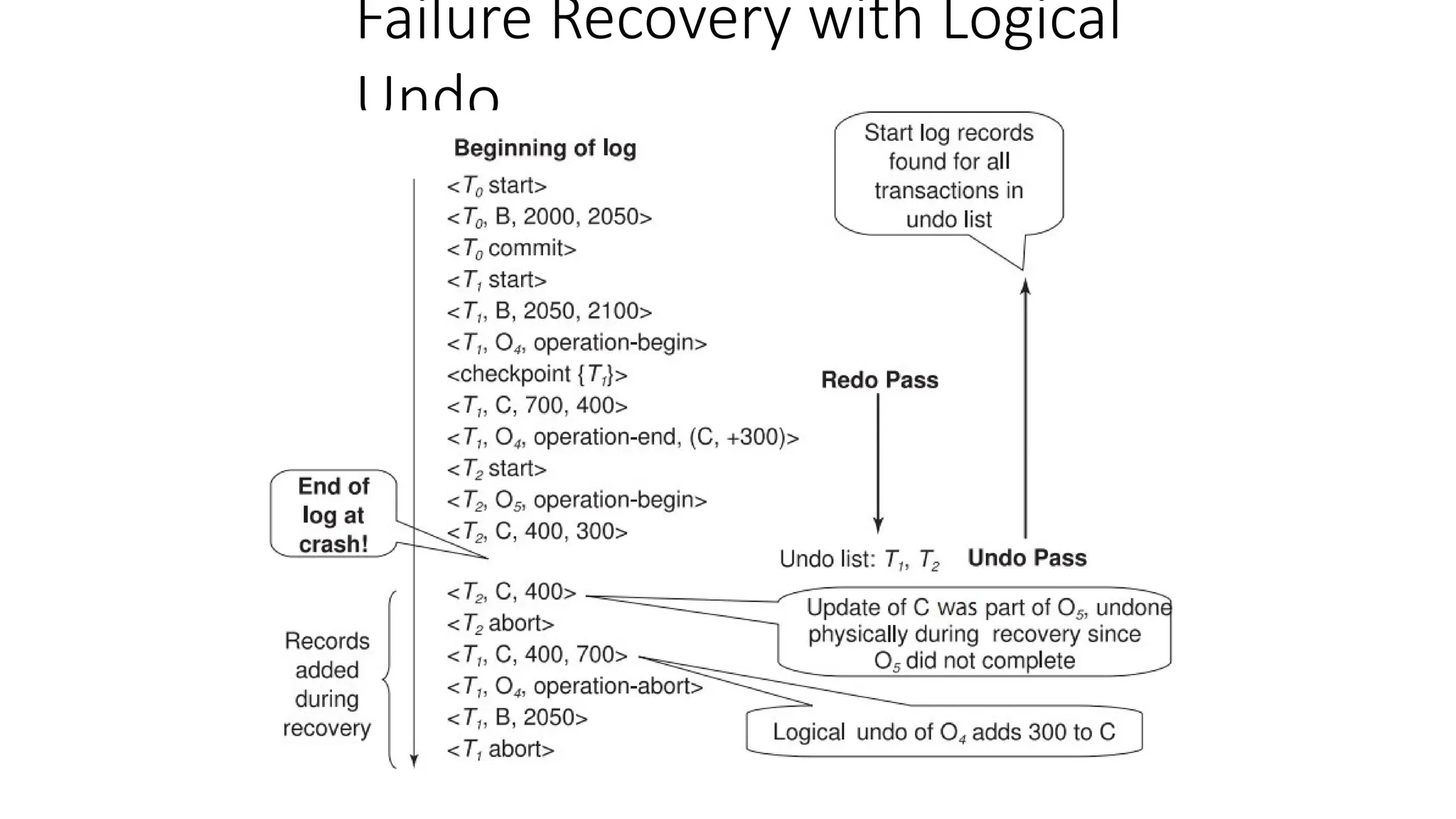
1. (Redo phase): Scan log forward from last < checkpoint L> record till end of log
1. Repeat history by physically redoing all updates of all transactions,
2. Create an undo-list during the scan as follows
 undo-list is set to L initially
 Whenever <Ti start> is found Ti is added to undo-list
 Whenever <Ti commit> or <Ti abort> is found, Ti is deleted from undo-list
This brings database to state as of crash, with committed as well as uncommitted
transactions having been redone
Now undo-list contains transactions that are incomplete, that is, have neither
committed nor been fully rolled back

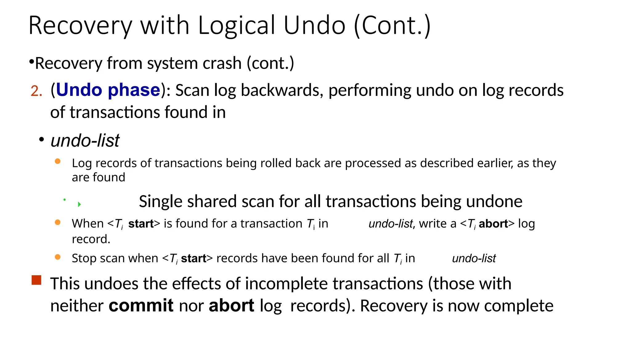
Recovery with Logical Undo (Cont.)
•Recovery from system crash (cont.)
2. (Undo phase): Scan log backwards, performing undo on log records
of transactions found in
• undo-list
 Log records of transactions being rolled back are processed as described earlier, as they
are found
•  Single shared scan for all transactions being undone
 When <Ti start> is found for a transaction Ti in undo-list, write a <Ti abort> log
record.
 Stop scan when <Ti start> records have been found for all Ti in undo-list
 This undoes the effects of incomplete transactions (those with
neither commit nor abort log records). Recovery is now complete

UPDATED UNIT 4 DBMS NOTES ECE DS SRM 21 Reg

More Related Content

Similar to UPDATED UNIT 4 DBMS NOTES ECE DS SRM 21 Reg

Recently uploaded

UPDATED UNIT 4 DBMS NOTES ECE DS SRM 21 Reg