primal and dual problem

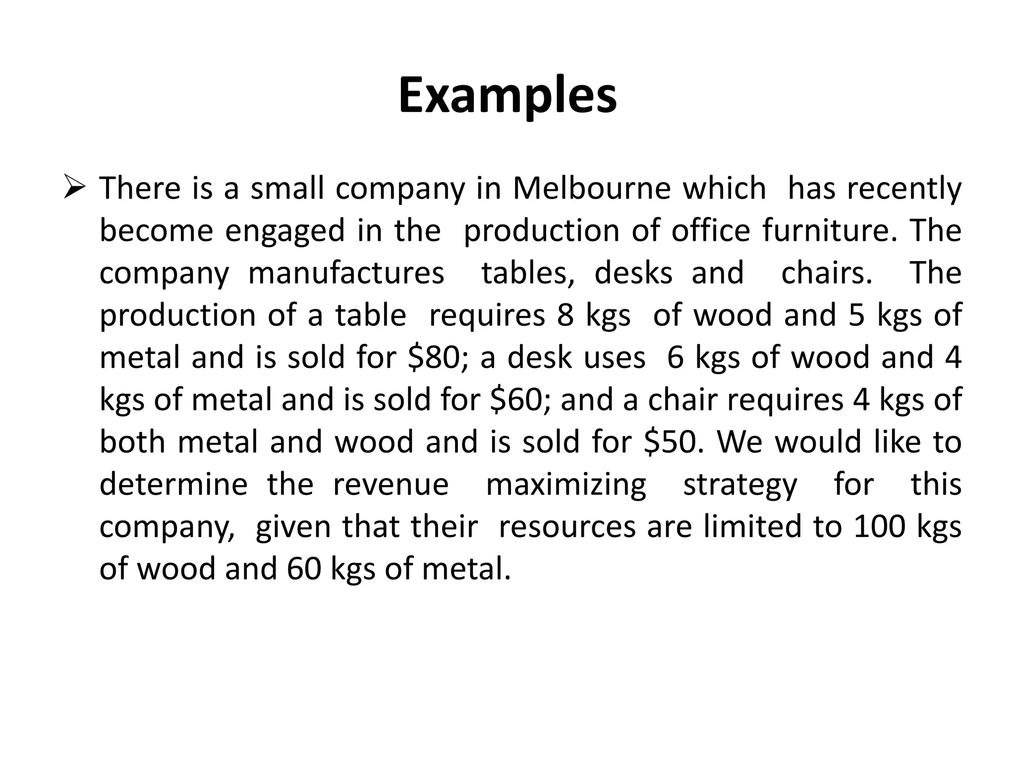
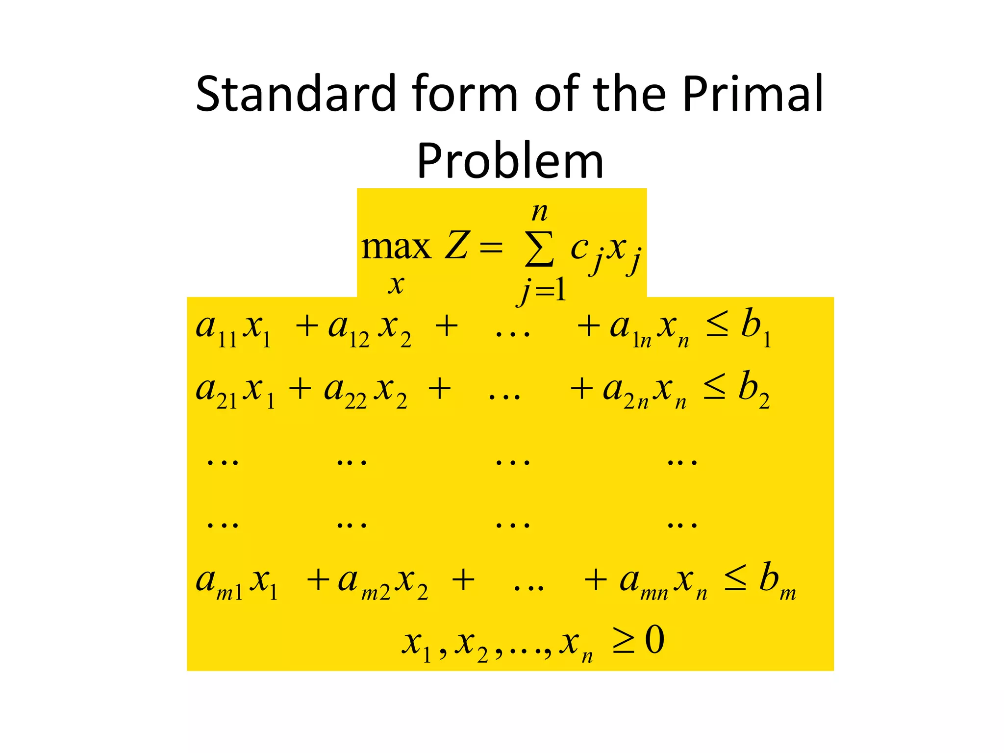
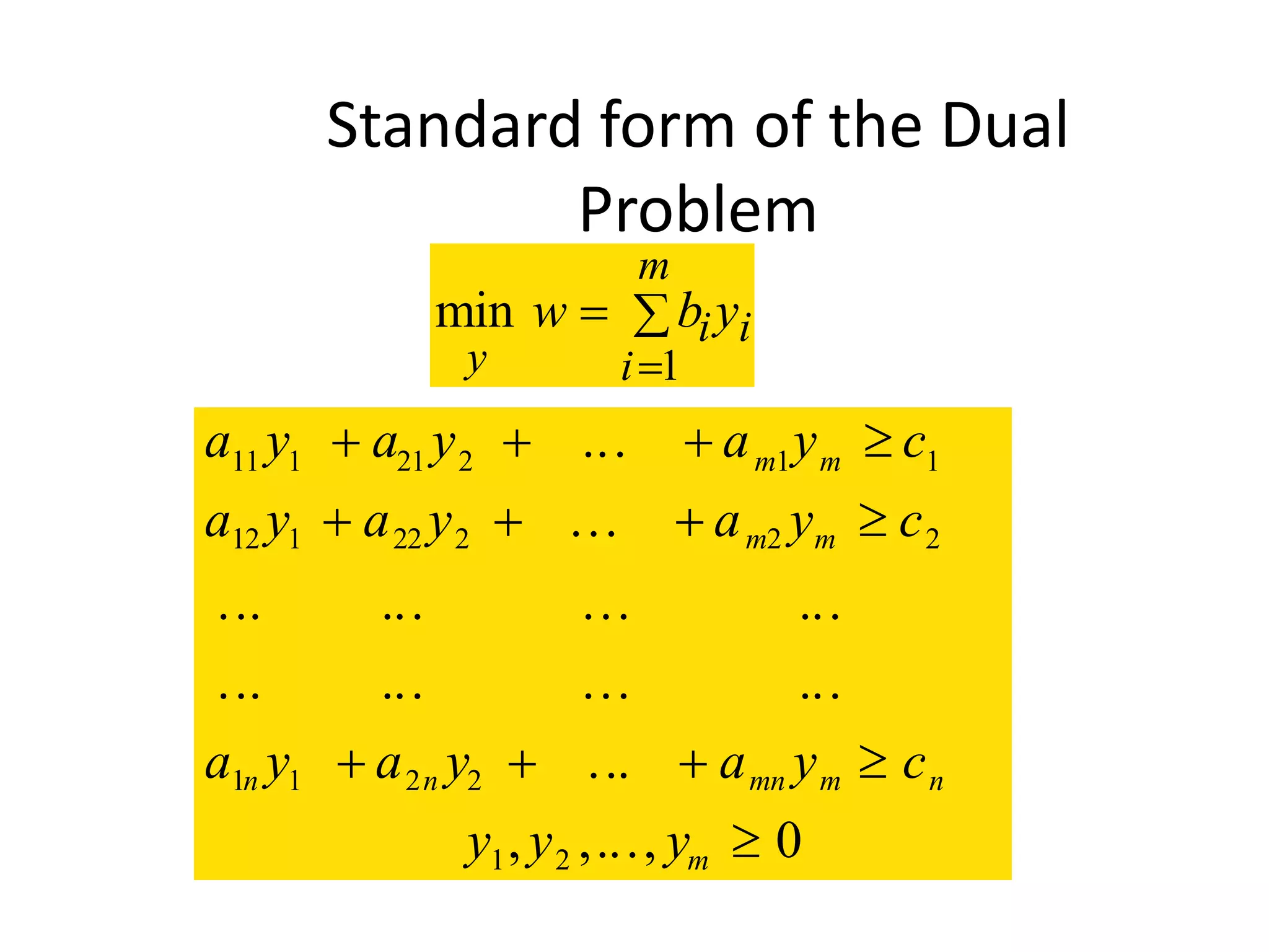
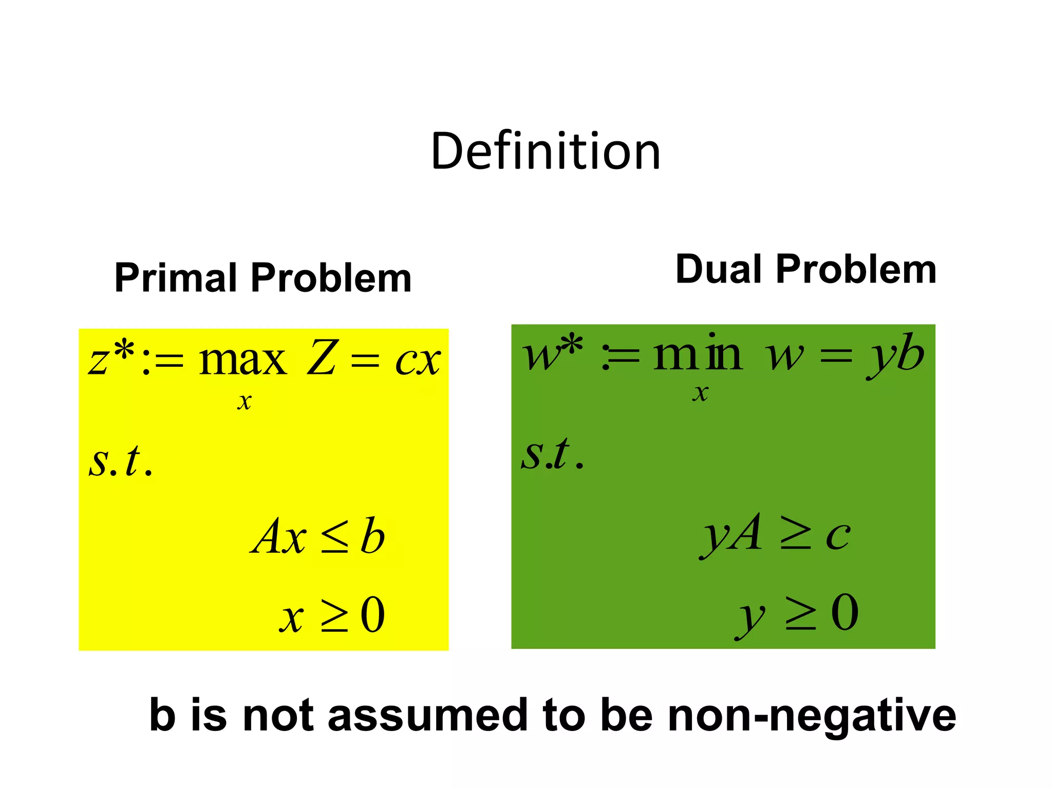
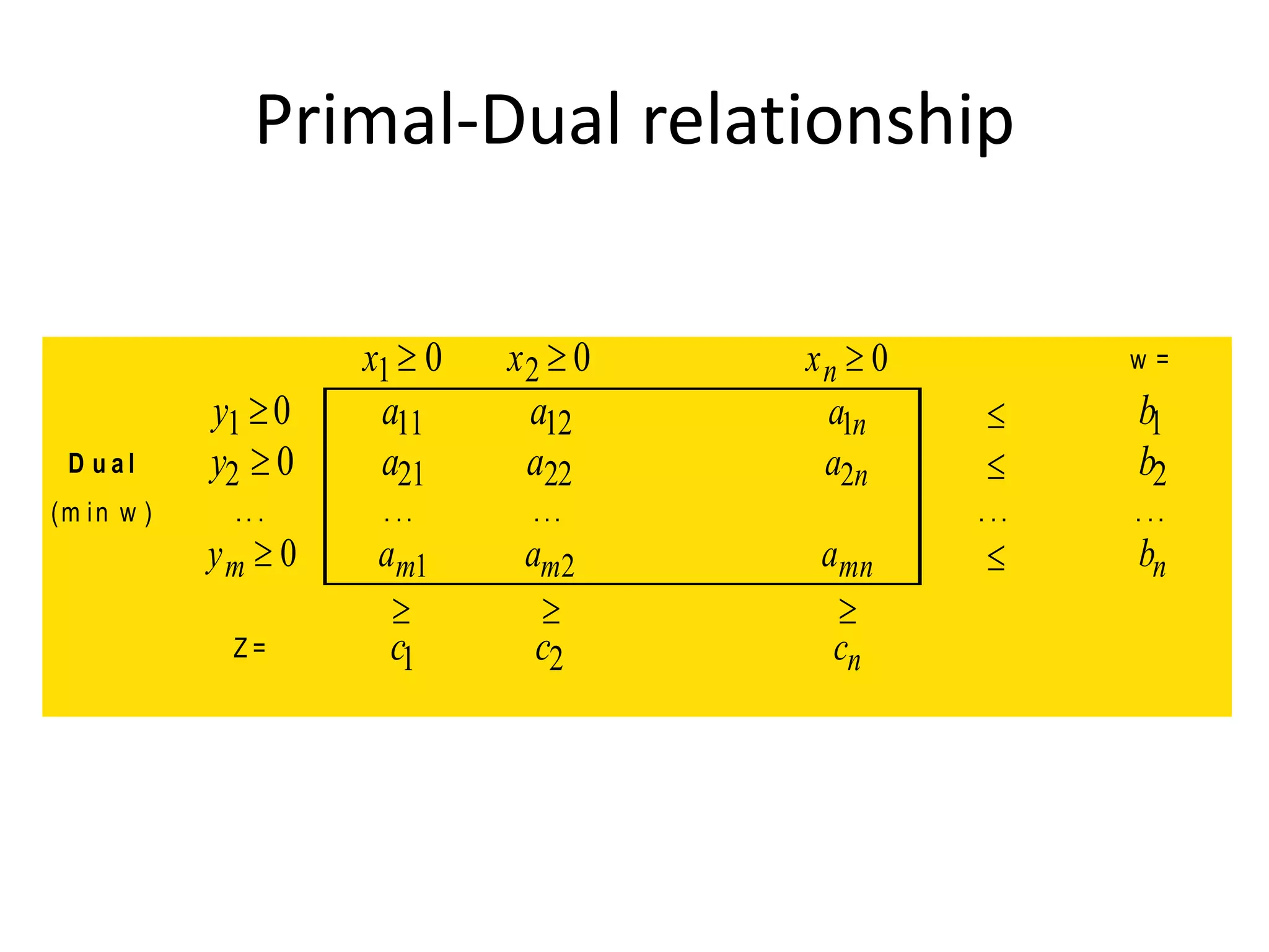
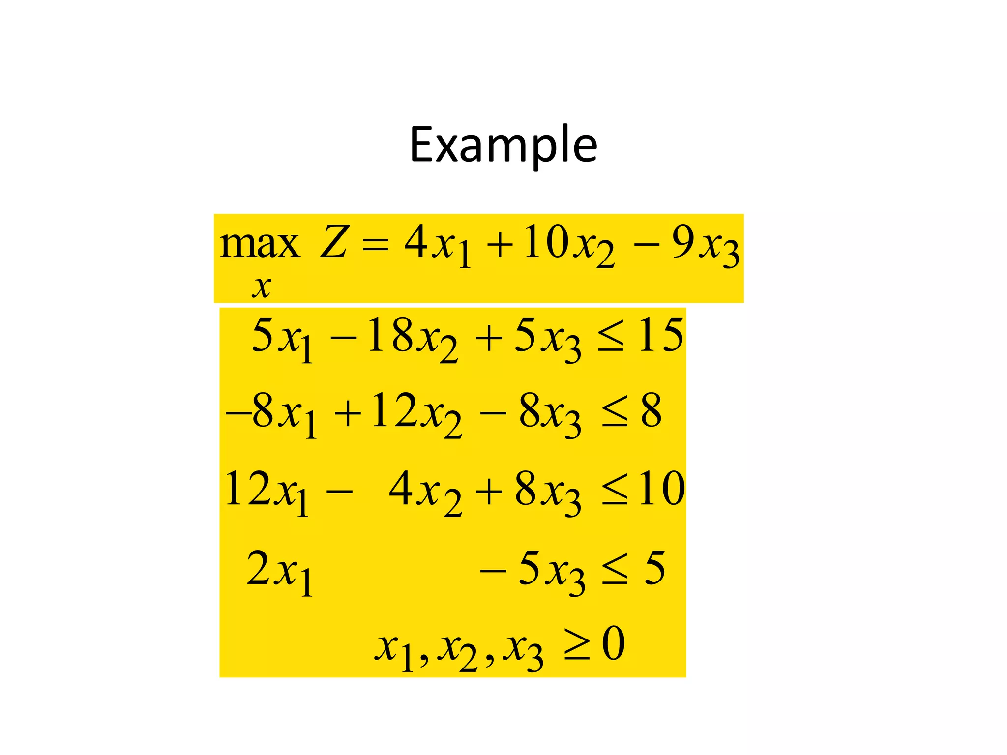
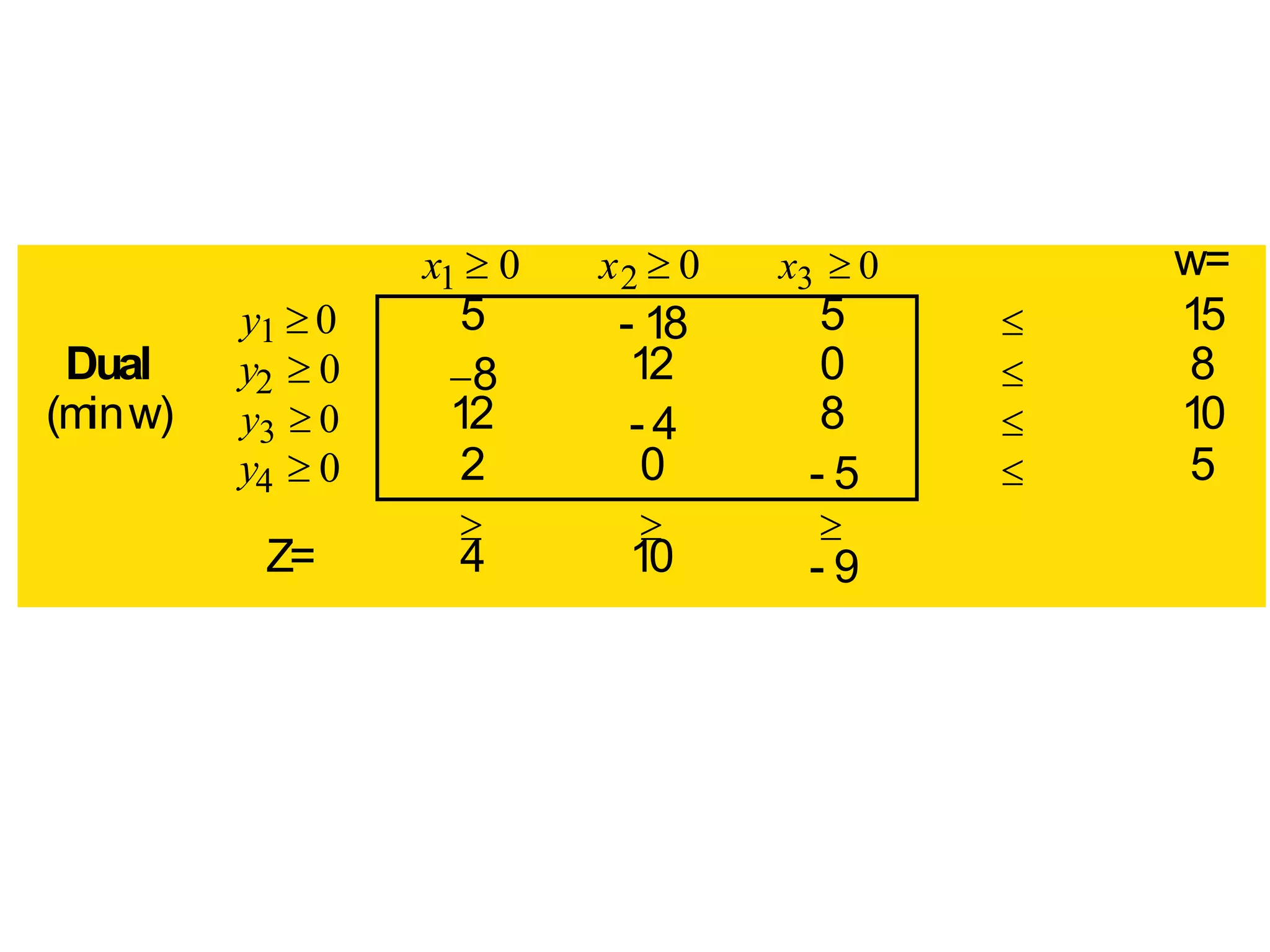
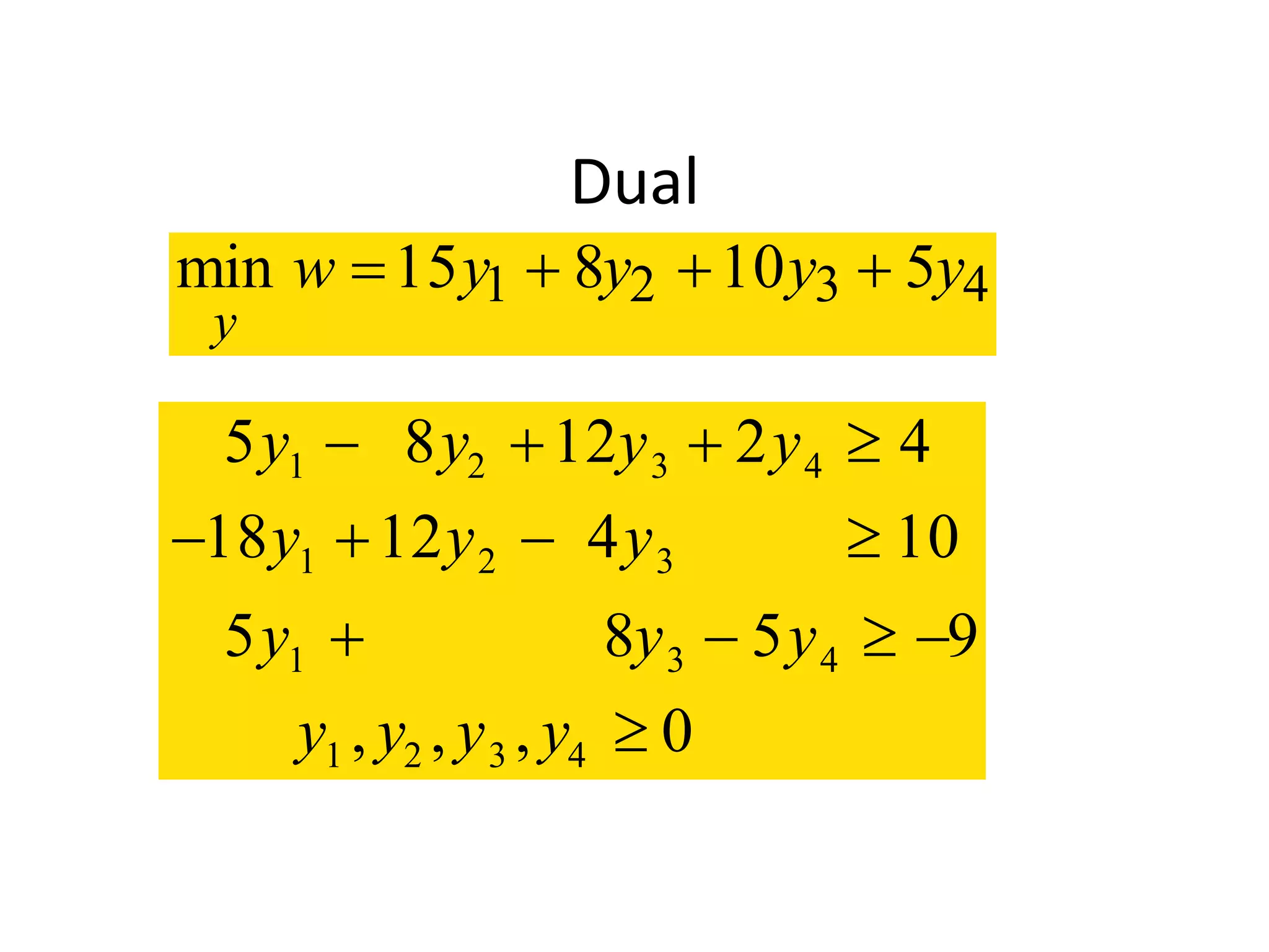
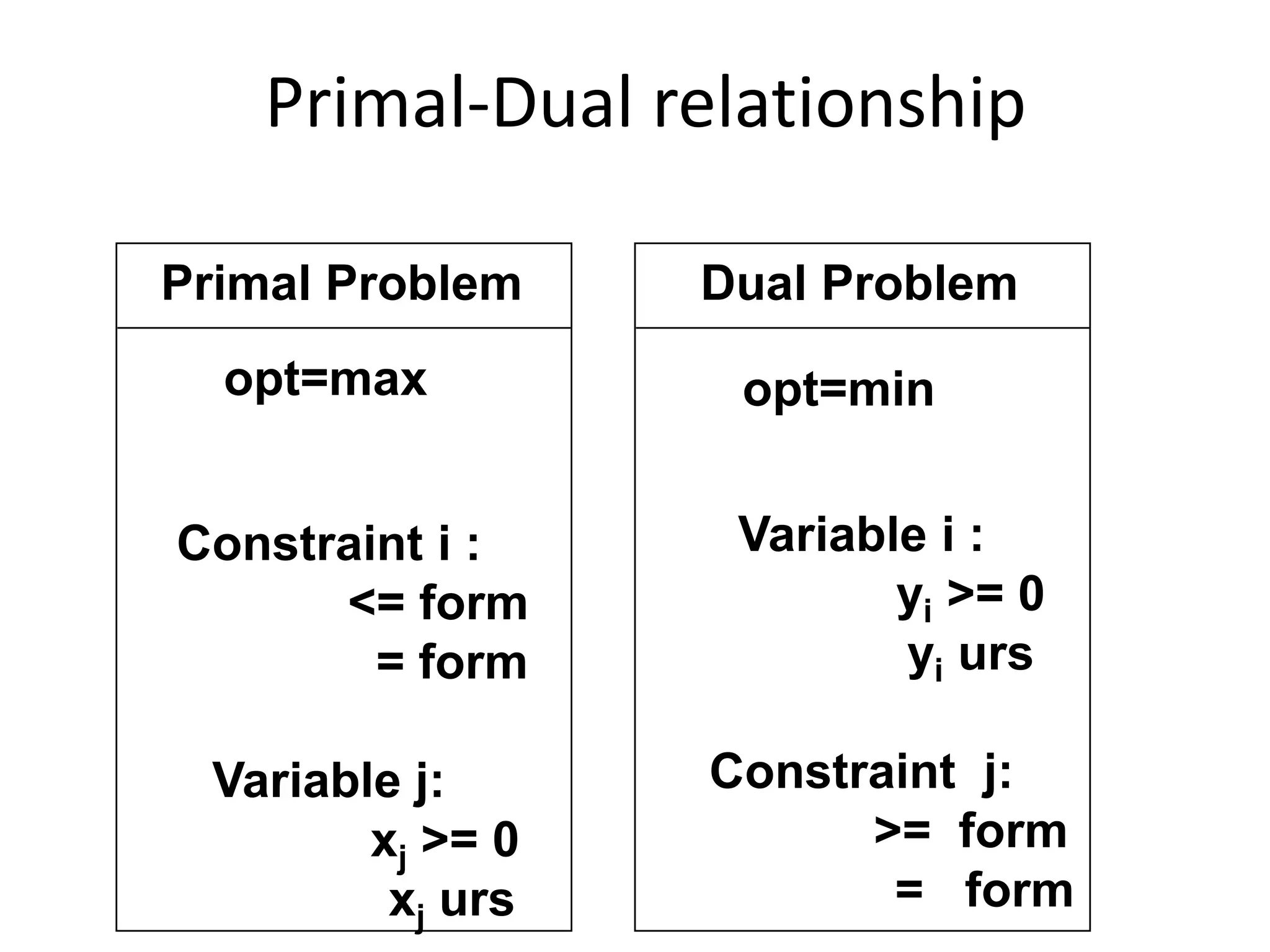
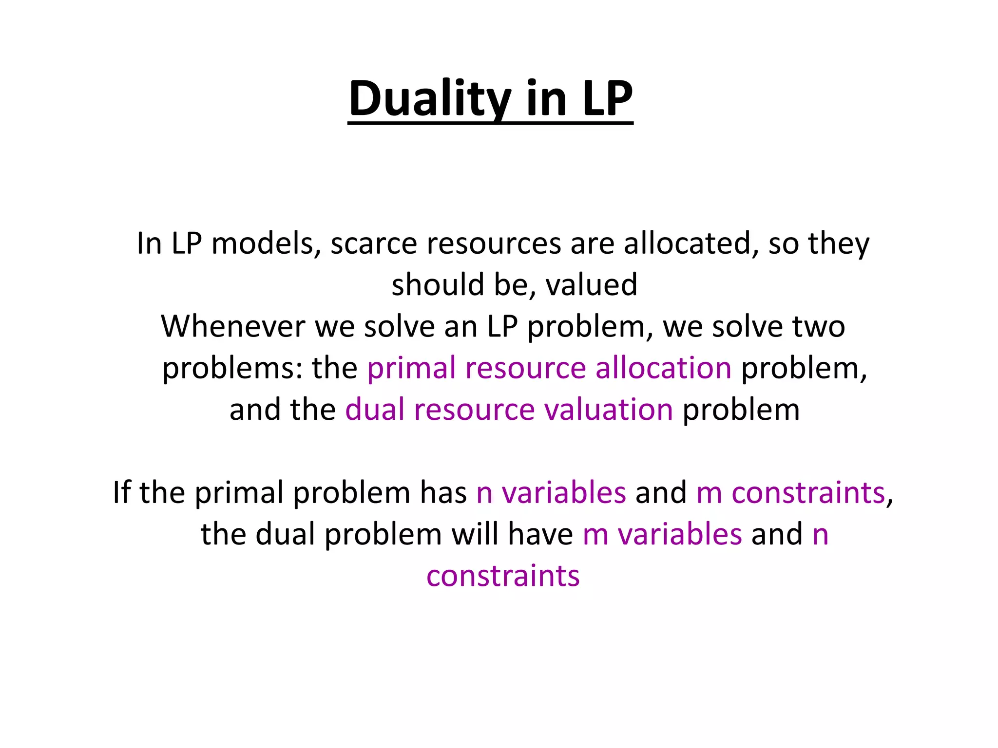
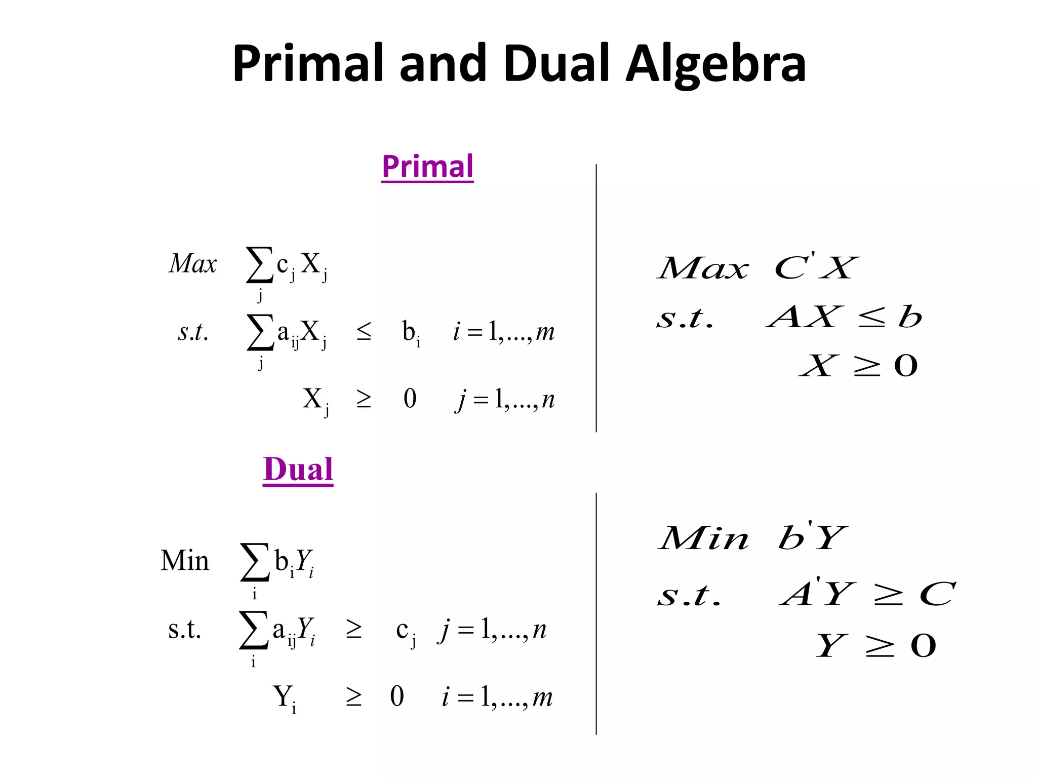
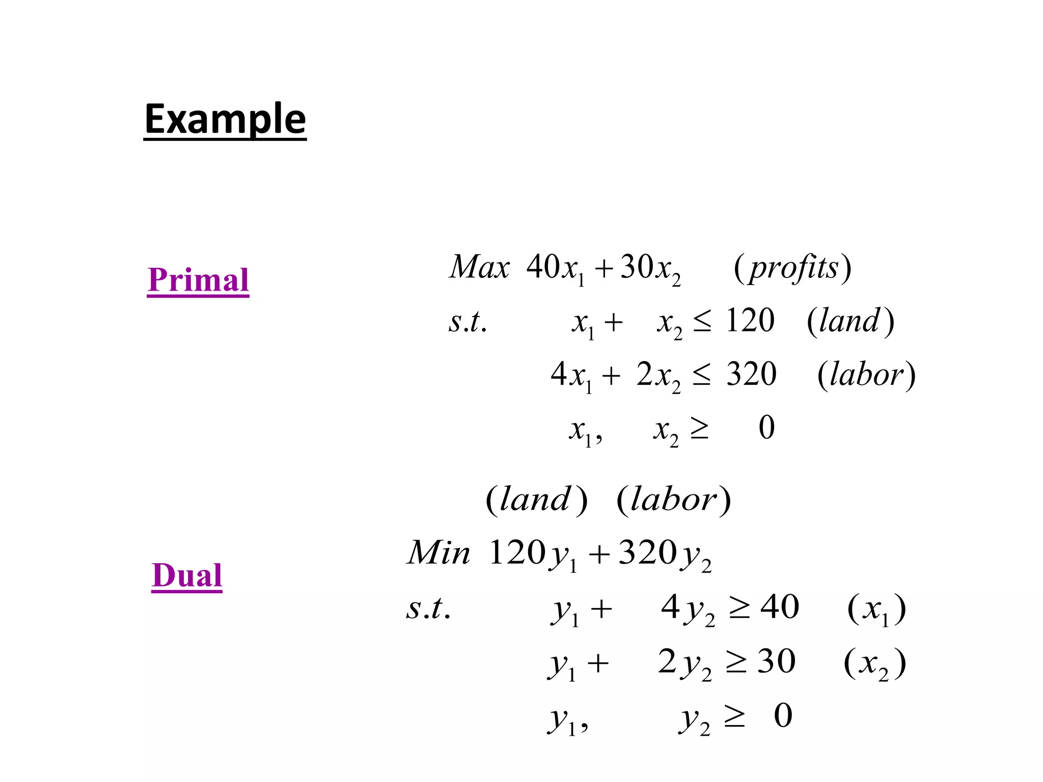
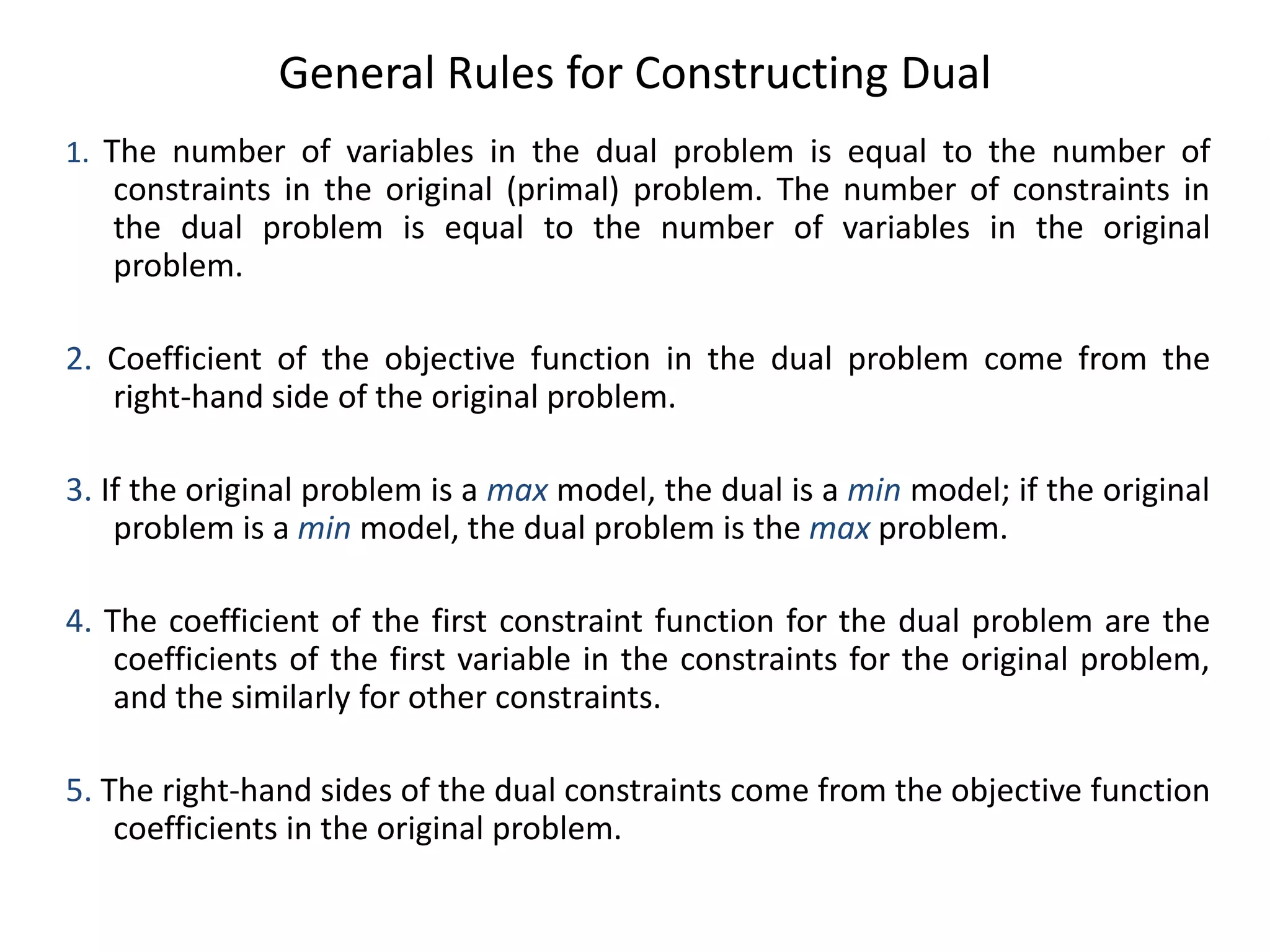
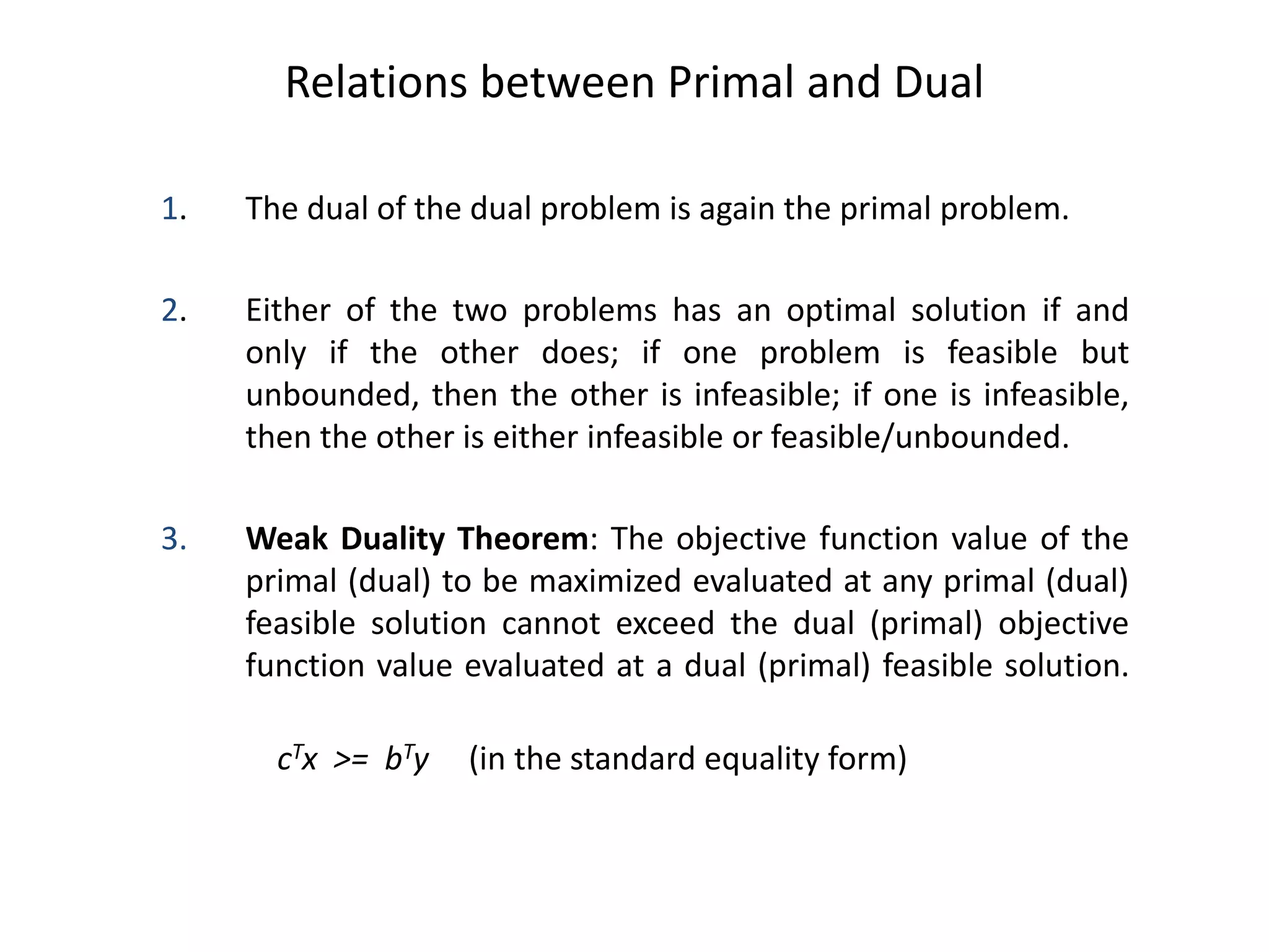
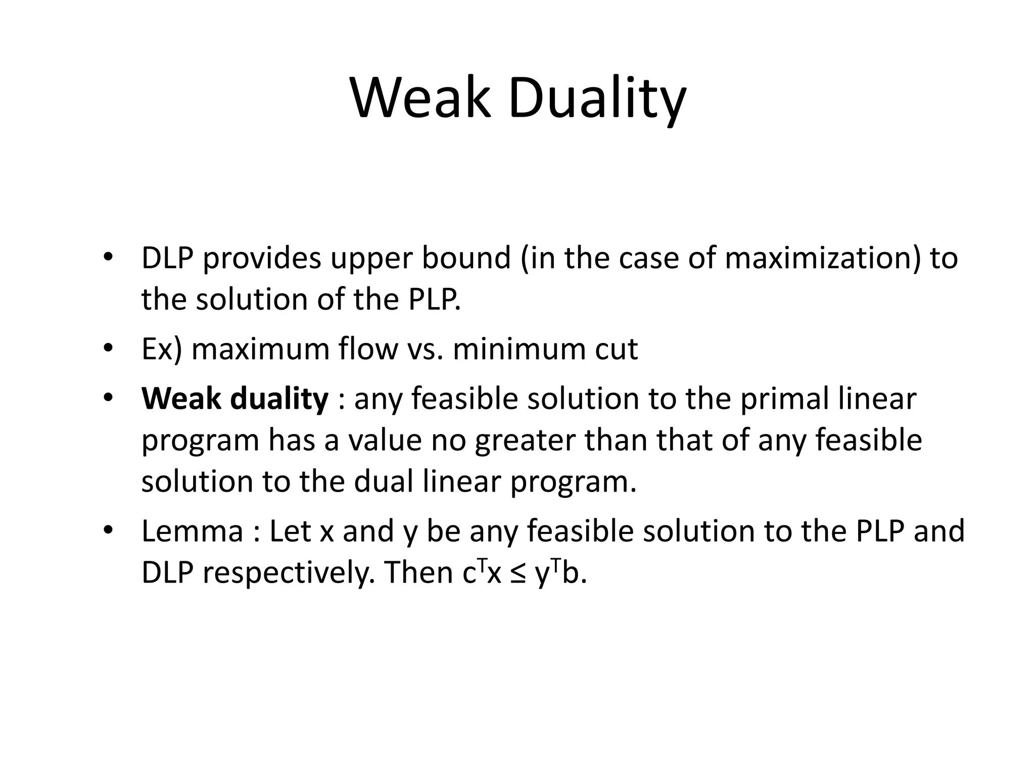
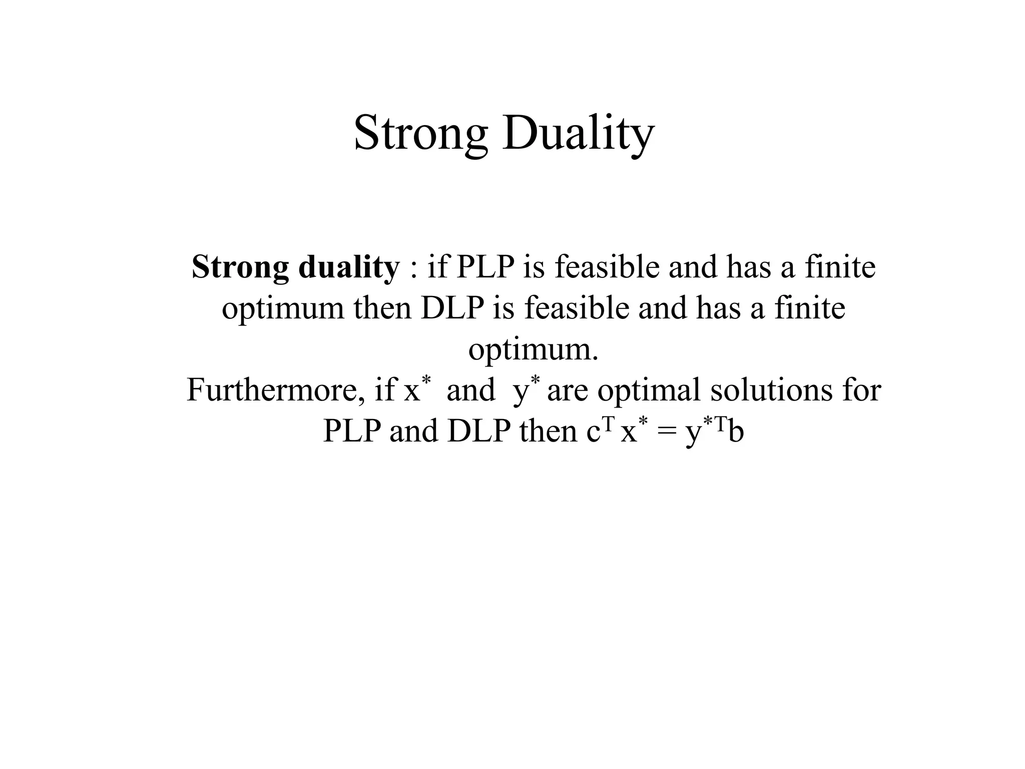
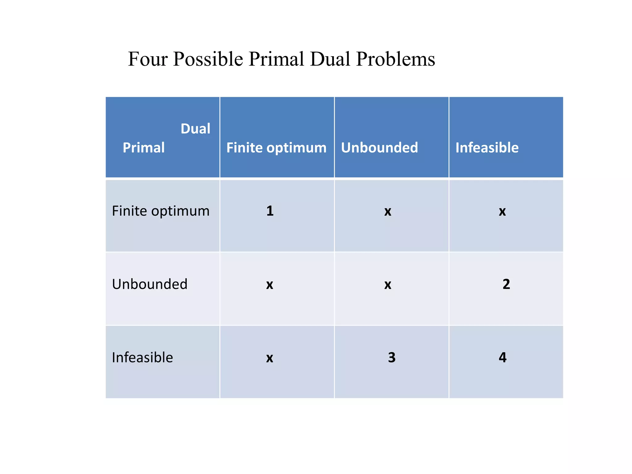
PRIMAL & DUAL
PROBLEMS,THEIR INTER
RELATIONSHIP
PREPARED BY:
130010119042 –KHAMBHAYATA MAYUR
130010119045 – KHANT VIJAY
130010119047 – LAD YASH A.
SUBMITTED TO:
PROF. S.R.PANDYA

CONTENT:
 Duality Theory
 Examples
 Standard form of the Dual Problem
 Definition
 Primal-Dual relationship
 Duality in LP
 General Rules for Constructing Dual
 Strong Dual
 Weak Dual

Duality Theory
 The theory of duality is a very elegant and important
concept within the field of operations research. This
theory was first developed in relation to linear
programming, but it has many applications, and
perhaps even a more natural and intuitive
interpretation, in several related areas such as
nonlinear programming, networks and game theory.

 The notion of duality within linear programming asserts
that every linear program has associated with it a
related linear program called its dual. The original
problem in relation to its dual is termed the primal.
 it is the relationship between the primal and its dual,
both on a mathematical and economic level, that is
truly the essence of duality theory.
Duality Theory (continue…)

Examples
 There is a small company in Melbourne which has recently
become engaged in the production of office furniture. The
company manufactures tables, desks and chairs. The
production of a table requires 8 kgs of wood and 5 kgs of
metal and is sold for $80; a desk uses 6 kgs of wood and 4
kgs of metal and is sold for $60; and a chair requires 4 kgs of
both metal and wood and is sold for $50. We would like to
determine the revenue maximizing strategy for this
company, given that their resources are limited to 100 kgs
of wood and 60 kgs of metal.

Standard form of the Primal
Problem
a x a x a x b
a x a x a x b
a x a x a x b
x x x
n n
n n
m m mn n m
n
11 1 12 2 1 1
21 1 22 2 2 2
1 1 2 2
1 2 0
   
   
   

...
...
... ... ... ...
... ... ... ...
...
, ,...,
max
x
j j
j
n
Z c x 
1

Standard form of the Dual
Problem
a y a y a y c
a y a y a y c
a y a y a y c
y y y
m m
m m
n n mn m n
m
11 1 21 2 1 1
12 1 22 2 2 2
1 1 2 2
1 2 0
   
   
   

...
...
... ... ... ...
... ... ... ...
...
, ,...,
min
y
i
i
m
iw b y 
1

Definition
z Z cx
s t
Ax b
x
x
*: max
. .
 

 0
w* : min
x
w  yb
s.t.
yA  c
y  0
Primal Problem Dual Problem
b is not assumed to be non-negative

Primal-Dual relationship
x1 0 x2 0 xn  0 w =
y1 0 a11 a12 a n1  b1
D u a l y2 0 a21 a22 a n2  b2
(m in w ) .. . . .. ... . .. . . .
ym  0 am1 am2 amn  bn
  
Z = c1 c2 cn

Example
5 18 5 15
8 12 8 8
12 4 8 10
2 5 5
0
1 2 3
1 2 3
1 2 3
1 3
1 2 3
x x x
x x x
x x x
x x
x x x
  
   
  
 
, ,
max
x
Z x x x  4 10 91 2 3

x1 0 x2 0 x3 0 w=
y1 0 5 - 18 5  15
Dual y2 0 8 12 0  8
(minw) y3 0 12 - 4 8  10
y4 0 2 0 - 5  5
  
Z= 4 10 - 9

Dual
5 8 12 2 4
18 12 4 10
5 8 5 9
0
1 2 3 4
1 2 3
1 3 4
1 2 3 4
y y y y
y y y
y y y
y y y y
   
   
   
, , ,
min
y
w y y y y   15 8 10 51 2 3 4

d x ei
i
k
i

 
1
d x e
d x e
i
i
k
i
i
i
k
i


 
 
1
1
d x e
d x e
i
i
k
i
i
i
k
i





  
1
1
Standard form!

Primal-Dual relationship
Primal Problem
opt=max
Constraint i :
<= form
= form
Variable j:
xj >= 0
xj urs
opt=min
Dual Problem
Variable i :
yi >= 0
yi urs
Constraint j:
>= form
= form

Duality in LP
In LP models, scarce resources are allocated, so they
should be, valued
Whenever we solve an LP problem, we solve two
problems: the primal resource allocation problem,
and the dual resource valuation problem
If the primal problem has n variables and m constraints,
the dual problem will have m variables and n
constraints

Primal and Dual Algebra
Primal
j j
j
ij j i
j
j
c X
. . a X b 1,...,
X 0 1,...,
Max
s t i m
j n
 
 


Dual
i
i
ij j
i
i
Min b
s.t. a c 1,...,
Y 0 1,...,
i
i
Y
Y j n
i m
 
 


'
. .
0
Max C X
s t X b
X





'
'
. .
0
Min b Y
s t AY C
Y







Example
1 2
1 2
1 2
1 2
40 30 ( )
. . 120 ( )
4 2 320 ( )
, 0
Max x x profits
s t x x land
x x labor
x x
  
    
   
  

 
 

1 2
1 2 1
1 2 2
1 2
( ) ( )
120 320
. . 4 40 ( )
2 30 ( )
, 0
land labor
Min y y
s t y y x
y y x
y y
 

  
  
  

 
 

Primal
Dual

General Rules for Constructing Dual
1. The number of variables in the dual problem is equal to the number of
constraints in the original (primal) problem. The number of constraints in
the dual problem is equal to the number of variables in the original
problem.
2. Coefficient of the objective function in the dual problem come from the
right-hand side of the original problem.
3. If the original problem is a max model, the dual is a min model; if the original
problem is a min model, the dual problem is the max problem.
4. The coefficient of the first constraint function for the dual problem are the
coefficients of the first variable in the constraints for the original problem,
and the similarly for other constraints.
5. The right-hand sides of the dual constraints come from the objective function
coefficients in the original problem.

Relations between Primal and Dual
1. The dual of the dual problem is again the primal problem.
2. Either of the two problems has an optimal solution if and
only if the other does; if one problem is feasible but
unbounded, then the other is infeasible; if one is infeasible,
then the other is either infeasible or feasible/unbounded.
3. Weak Duality Theorem: The objective function value of the
primal (dual) to be maximized evaluated at any primal (dual)
feasible solution cannot exceed the dual (primal) objective
function value evaluated at a dual (primal) feasible solution.
cTx >= bTy (in the standard equality form)

Relations between Primal and Dual (continued)
4. Strong Duality Theorem: When there is an optimal solution, the
optimal objective value of the primal is the same as the optimal
objective value of the dual.
cTx* = bTy*

Weak Duality
• DLP provides upper bound (in the case of maximization) to
the solution of the PLP.
• Ex) maximum flow vs. minimum cut
• Weak duality : any feasible solution to the primal linear
program has a value no greater than that of any feasible
solution to the dual linear program.
• Lemma : Let x and y be any feasible solution to the PLP and
DLP respectively. Then cTx ≤ yTb.

Strong duality : if PLP is feasible and has a finite
optimum then DLP is feasible and has a finite
optimum.
Furthermore, if x* and y* are optimal solutions for
PLP and DLP then cT x* = y*Tb
Strong Duality

Four Possible Primal Dual Problems
Dual
Primal Finite optimum Unbounded Infeasible
Finite optimum 1 x x
Unbounded x x 2
Infeasible x 3 4

primal and dual problem

More Related Content

What's hot

Similar to primal and dual problem

More from Yash Lad

Recently uploaded

In this document

primal and dual problem