Downloaded 34 times
![OPERATING SYSTEM NOTES
UNIT-III
[Process Scheduling : Scheduling criteria, preemptive & non-preemptive scheduling, scheduling algorithms]
INTRODUCTION:
In a single-processor system, only one process can run at a time; any others must wait until the CPU
is free. The objective of multiprogramming is to have some process running at all times, to
maximize CPU utilization. In this scheme, several processes are kept in memory at one time.
Process execution consists of a cycle of CPU execution and I/O wait. Process execution begins with
a CPU burst. That is followed by an I/O burst, which is followed by another CPU burst, then
another I/O burst, and so on. Eventually, the final CPU burst ends with a system request to
terminate execution.
When one process has to wait, the CPU becomes idle. Then the operating system selects one of the
processes in the ready queue to be executed. The selection process is carried out by the short-term
scheduler (CPU Scheduler).
Another component involved in the CPU-scheduling function is the dispatcher. The dispatcher is
the module that gives control of the CPU to the process selected by the short-term scheduler. This
Provided By Shipra Swati](https://image.slidesharecdn.com/osunit-iiinotes-181017042959/75/Operating-System-Process-Scheduling-1-2048.jpg)
![OPERATING SYSTEM NOTES
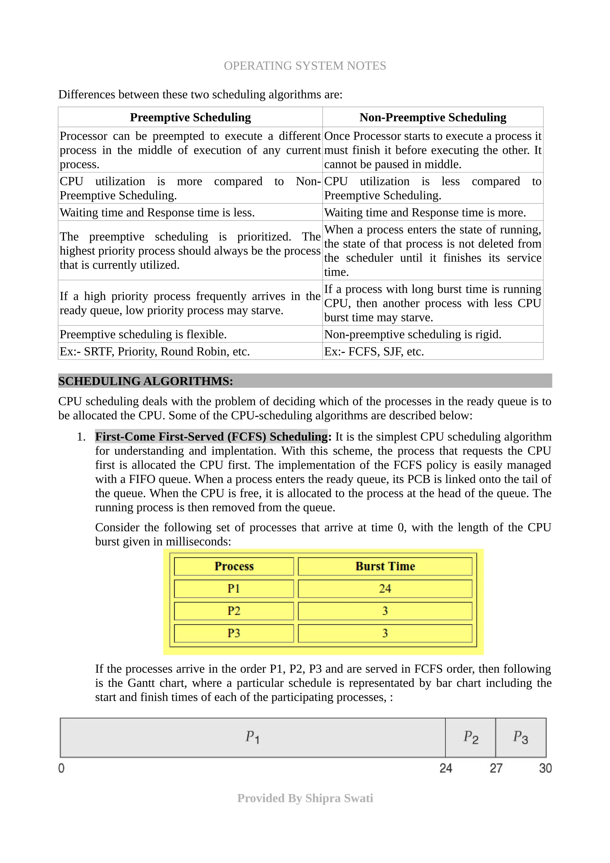
By comparison, if we were using the FCFS scheduling scheme, the average waiting time
would be 10.25 milliseconds.
SJF can be proven to be the fastest scheduling algorithm, but it suffers from one
important problem: How to know the required CPU time in advance?
It is easy to implement in Batch systems where required CPU time is known in advance, but
impossible to implement in interactive systems where required CPU time is not known.
The SJF algorithm can be either preemptive or nonpreemptive. The choice arises when a
new process arrives at the ready queue while a previous process is still executing. The next
CPU burst of the newly arrived process may be shorter than what is left of the currently
executing process. A preemptive SJF algorithm will preempt the currently executing
process, whereas a non-preemptive SJF algorithm will allow the currently running process
to finish its CPU burst. Preemptive SJF scheduling is sometimes called shortest-
remaining-time-first scheduling. As an example, consider the following four processes,
with the length of the CPU burst given in milliseconds:
If the processes arrive at the ready queue at the times shown and need the indicated burst
times, then the resulting preemptive SJF schedule is as depicted in the following Gantt
chart:
Process P1 is started at time 0, since it is the only process in the queue. Process P2 arrives at
time 1. The remaining time for process P1 (7 milliseconds) is larger than the time required
by process P2 (4 milliseconds), so process P1 is preempted, and process P2 is scheduled.
The average waiting time for this example is:
[(10- 1) + (1 - 1) + (17- 2) +(5-3)]/ 4 = 26/4 = 6.5 milliseconds.
Nonpreemptive SJF scheduling would result in an average waiting time of 7.75 milliseconds
and FCFS will have waiting time of 8.75 ms.
Provided By Shipra Swati](https://image.slidesharecdn.com/osunit-iiinotes-181017042959/75/Operating-System-Process-Scheduling-5-2048.jpg)
![OPERATING SYSTEM NOTES
UNIT-III
[Process Scheduling : Scheduling criteria, preemptive & non-preemptive scheduling, scheduling algorithms]
INTRODUCTION:
In a single-processor system, only one process can run at a time; any others must wait until the CPU
is free. The objective of multiprogramming is to have some process running at all times, to
maximize CPU utilization. In this scheme, several processes are kept in memory at one time.
Process execution consists of a cycle of CPU execution and I/O wait. Process execution begins with
a CPU burst. That is followed by an I/O burst, which is followed by another CPU burst, then
another I/O burst, and so on. Eventually, the final CPU burst ends with a system request to
terminate execution.
When one process has to wait, the CPU becomes idle. Then the operating system selects one of the
processes in the ready queue to be executed. The selection process is carried out by the short-term
scheduler (CPU Scheduler).
Another component involved in the CPU-scheduling function is the dispatcher. The dispatcher is
the module that gives control of the CPU to the process selected by the short-term scheduler. This
Provided By Shipra Swati](https://crownmelresort.com/image.slidesharecdn.com/osunit-iiinotes-181017042959/75/Operating-System-Process-Scheduling-1-2048.jpg)


![OPERATING SYSTEM NOTES
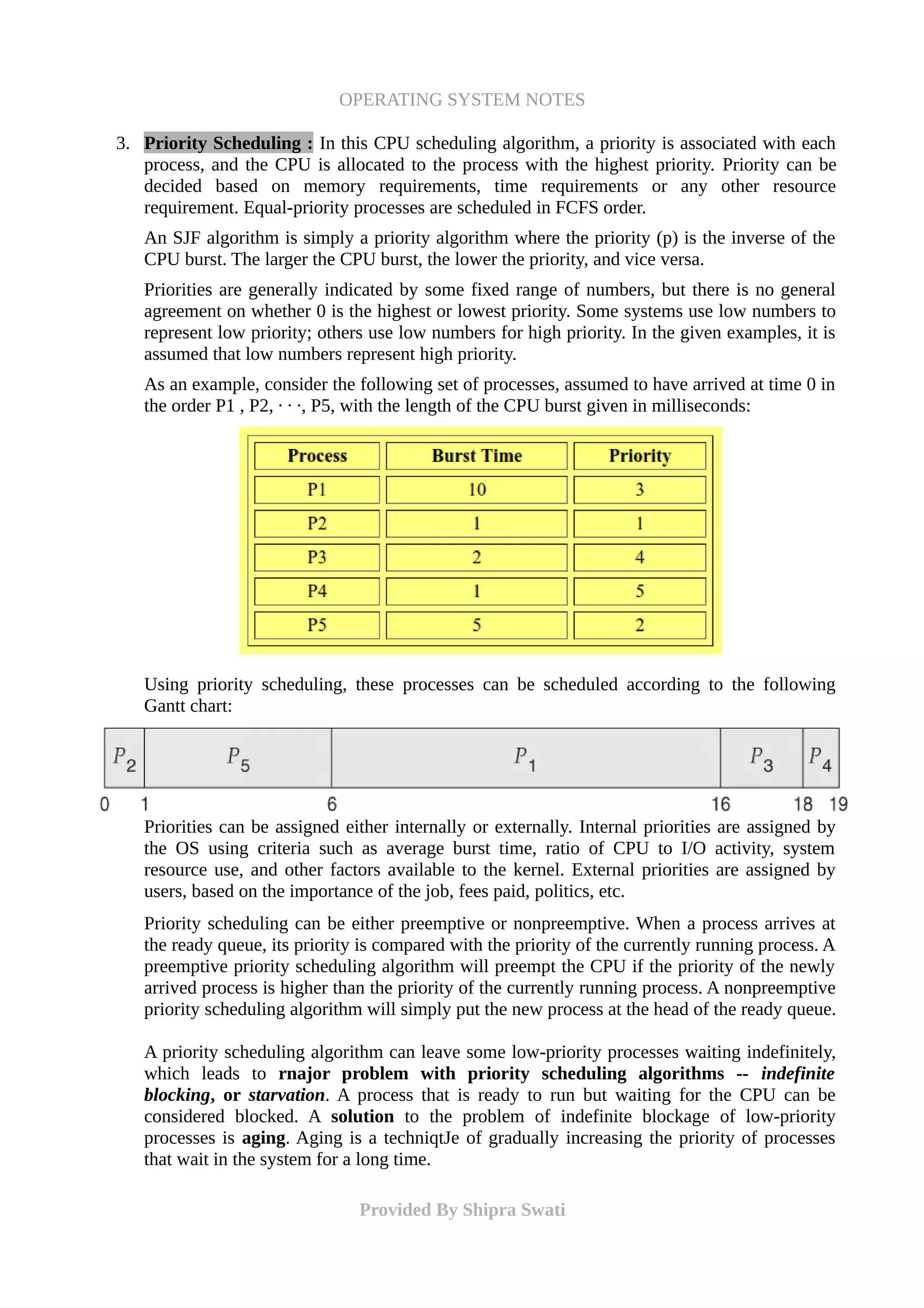
By comparison, if we were using the FCFS scheduling scheme, the average waiting time
would be 10.25 milliseconds.
SJF can be proven to be the fastest scheduling algorithm, but it suffers from one
important problem: How to know the required CPU time in advance?
It is easy to implement in Batch systems where required CPU time is known in advance, but
impossible to implement in interactive systems where required CPU time is not known.
The SJF algorithm can be either preemptive or nonpreemptive. The choice arises when a
new process arrives at the ready queue while a previous process is still executing. The next
CPU burst of the newly arrived process may be shorter than what is left of the currently
executing process. A preemptive SJF algorithm will preempt the currently executing
process, whereas a non-preemptive SJF algorithm will allow the currently running process
to finish its CPU burst. Preemptive SJF scheduling is sometimes called shortest-
remaining-time-first scheduling. As an example, consider the following four processes,
with the length of the CPU burst given in milliseconds:
If the processes arrive at the ready queue at the times shown and need the indicated burst
times, then the resulting preemptive SJF schedule is as depicted in the following Gantt
chart:
Process P1 is started at time 0, since it is the only process in the queue. Process P2 arrives at
time 1. The remaining time for process P1 (7 milliseconds) is larger than the time required
by process P2 (4 milliseconds), so process P1 is preempted, and process P2 is scheduled.
The average waiting time for this example is:
[(10- 1) + (1 - 1) + (17- 2) +(5-3)]/ 4 = 26/4 = 6.5 milliseconds.
Nonpreemptive SJF scheduling would result in an average waiting time of 7.75 milliseconds
and FCFS will have waiting time of 8.75 ms.
Provided By Shipra Swati](https://crownmelresort.com/image.slidesharecdn.com/osunit-iiinotes-181017042959/75/Operating-System-Process-Scheduling-5-2048.jpg)


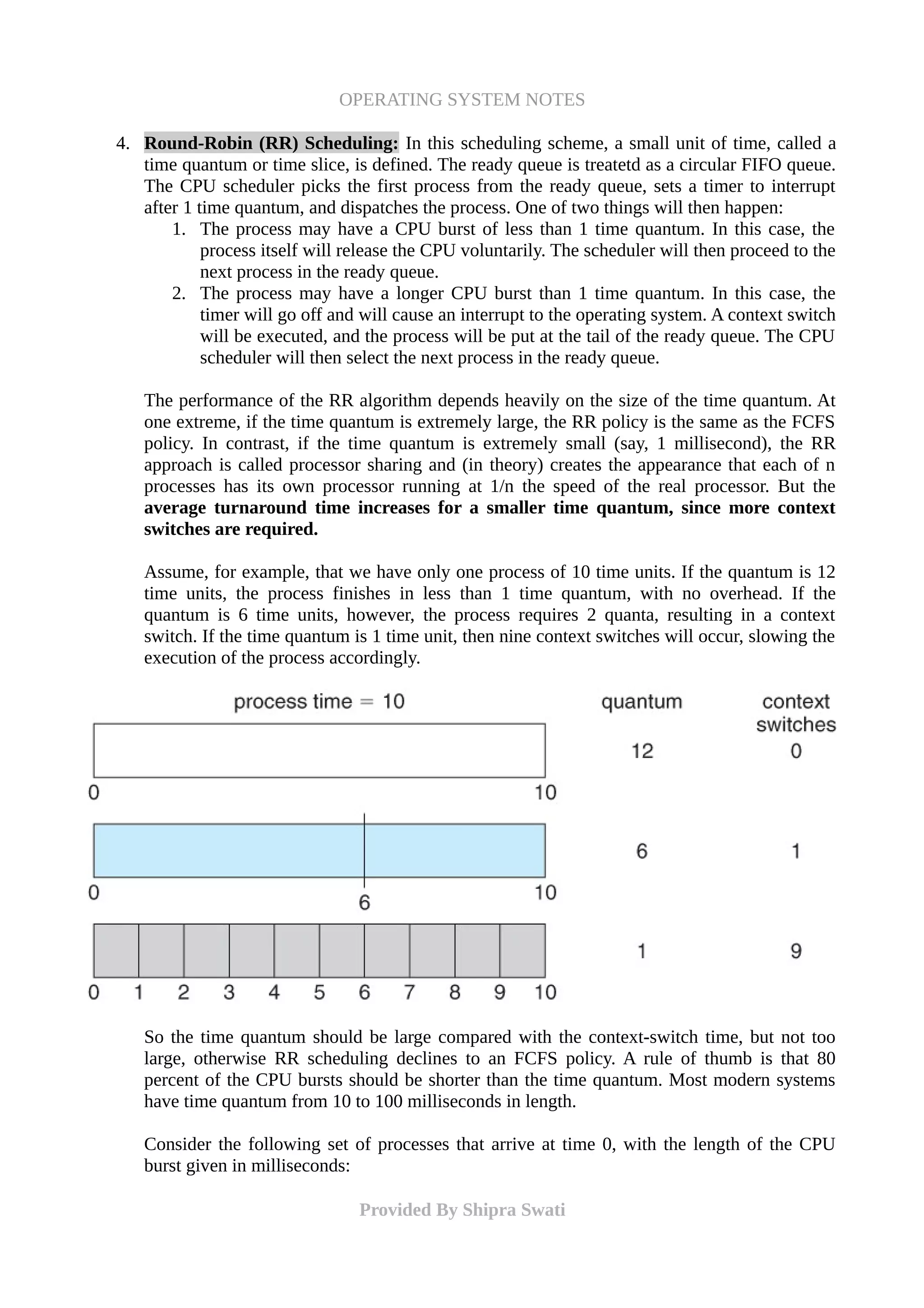
The document discusses process scheduling in operating systems, focusing on scheduling criteria, preemptive and non-preemptive scheduling, and various scheduling algorithms such as FCFS, SJF, priority scheduling, round-robin, multilevel queue, and multilevel feedback queue. It highlights the objectives of maximizing CPU utilization and throughput while minimizing turnaround time, waiting time, and response time. The document outlines the characteristics, advantages, and drawbacks of different scheduling methods and their impact on process management.


![SHS_Core_CAE_Q3_LE1 FOR THIRD [FINAL].pdf](https://cdn.slidesharecdn.com/ss_thumbnails/shscorecaeq3le1final-251116055110-e3081055-thumbnail.jpg?width=640&height=640&fit=bounds)


