NUMERICAL ANALYSIS: APPROXIMATION,ERRORS & OPERATORS
Numerical Analysis || Lecture Notes || Anup Kumar Giri 1
ROUNDING-OFF NUMBERS AND ERRORS
Two major techniques are used to solve any mathematical problem analytical and numerical. The analytical solution is
obtained in a compact form and generally it is free from error. On the other hand, numerical method is a technique which
is used to solve a problem with the help of computer or calculator. In general, the solution obtained by this method
contains some error. But, for some class of problems it is very difficult to obtain an analytical solution. For these problems
we generally use numerical methods.
Numerical methods are to provide practical procedures for obtaining the numerical solutions of problems to a specified
degree of accuracy. In numerical analysis, besides the study of the methods, one studies the errors involving in the methods
and in the final results.
APPROXIMATE NUMBER AND SIGNIFICANT FIGURES
In the decimal representation of a number, an approximate number may be defined as a number which is used as an
approximation to an exact number. Some numbers like 𝜋, 𝑒 and √2 are exact numbers, but they cannot be represented
exactly by a finite number of digits. If we express 𝜋, for example, in decimal form as 3.1416, then the number 3.1416 is
only an approximation to the true value of 𝜋 and it is termed an approximate number.
In the decimal representation of a number, a digit is said to be significant figure if it is either a non-zero digit or any
zero(s) lying between two non-zero digits are used as a placeholder, to indicate a retrained place. All other zeros used to
fix-up the position of the decimal point are not to be counted as significant digit or figure.
The number of significant digits in a number will be counted from the left-most non-zero digit towards right. Thus, the
numbers 0.7452 and 0.007452 both have four significant digits. Similarly, 0.00400307 has 6 significant digits, 0.4003001
has 7 significant digits and 0.30040000 has 8 significant digits.
EXAMPLE:
Find the number of significant figures in the numbers: (𝑎) 6.01203 (𝑏) 0.38002 (𝑐) 0.000032401 (𝑑) 82010000
Solution:
(a) 6.01203 = 0.601203 × 101
The number of significant figures is 6.
(b) 0.38002 = 0.38002 × 100
The number of significant figures is 5.
(c) 0.000032401 = 0.32401 × 10⁻⁴
The number of significant digits is 5.
(d) 82010000 = 0.8201 × 108
= 0.82010 × 108
= 0.820100 × 10⁸
The number of significant figures is 4 or 5 or 6. In such cases, the number of significant figures is not definite.
3.
NUMERICAL ANALYSIS: APPROXIMATION,ERRORS & OPERATORS
Numerical Analysis || Lecture Notes || Anup Kumar Giri 2
RULES OF ROUNDING-OFF
In rounding-off process the number is approximated to a very close number consisting of a smaller number of digits. In
that case, one or more digits are kept with the number, taken from left to right, and all other digits are discarded.
Let 𝑃 = 𝑎𝑛𝑎𝑛−1 ⋯ 𝑎2𝑎1𝑎0 ∙ 𝑎−1𝑎−2 ⋯ 𝑎−𝑘𝑎−(𝑘+1) ⋯ be a number in the decimal system, where each 𝑎𝑖 assumes one of
the values 0, 1, 2, ⋯ , 9 and 𝑎𝑛 ≠ 0.
Suppose we want to round-off the number 𝑃 to 𝑘 places of decimals.
RULE I:
If 𝑎−(𝑘+1) is one of the digits 0, 1, 2, 3, 4, then 𝑃 is rounded to 𝑎𝑛𝑎𝑛−1 ⋯ 𝑎2𝑎1𝑎0 ∙ 𝑎−1𝑎−2 ⋯ 𝑎−𝑘,
i.e. if the discarded digits constitute a number which is smaller than half the unit in the last decimal place that remains,
then the digits that remain do not change.
RULE II:
If 𝑎−(𝑘+1) is one of the digits 6, 7, 8, 9, then 𝑃 is rounded to 𝑎𝑛𝑎𝑛−1 ⋯ 𝑎2𝑎1𝑎0 ∙ 𝑎−1𝑎−2 ⋯ (𝑎−𝑘 + 1),
i.e. if the discarded digits constitute a number which is larger than half the unit in the last decimal place that remains, then
the last digit that is left is increased by one.
RULE III:
If 𝑎−(𝑘+1) = 5 which is followed by at least one non-zero digit, 𝑃 is rounded to 𝑎𝑛𝑎𝑛−1 ⋯ 𝑎2𝑎1𝑎0 ∙ 𝑎−1𝑎−2 ⋯ (𝑎−𝑘 + 1),
and if 𝑎−(𝑘+1) = 5, being the last non-zero digit, P is rounded to
(𝑖) 𝑎𝑛𝑎𝑛−1 ⋯ 𝑎2𝑎1𝑎0 ∙ 𝑎−1𝑎−2 ⋯ 𝑎−𝑘 when 𝑎−𝑘 is even, and
(𝑖𝑖) 𝑎𝑛𝑎𝑛−1 ⋯ 𝑎2𝑎1𝑎0 ∙ 𝑎−1𝑎−2 ⋯ (𝑎−𝑘 + 1) when 𝑎−𝑘 is odd.
i.e. If the discarded digits constitute a number which is equal to half the unit in the last decimal place that remains, then
the last digit that is half is increased by one, if it is odd, and is unchanged if it is even. This rule is often called a rule of
an even digit.
ILLUSTRATION:
Exact Number
Round-off number to six
significant figures
Remark
26.0123728 26.0124 (added 1 in the last digit)
23.12432605 23.1243 (last digit remains unchanged)
30.455354 30.4554 (added 1 in the last digit)
19.652453 19.6525 (added 1 in the last digit)
126.3545 126.354 (last digit remains unchanged)
34.44275 34.4428 (added 1 in the last digit to make even digit)
4.
NUMERICAL ANALYSIS: APPROXIMATION,ERRORS & OPERATORS
Numerical Analysis || Lecture Notes || Anup Kumar Giri 3
SOURCES OF ERROR
It is well known that the solution of a problem obtained by numerical method contains some errors. But our intension is
to minimize the error. To minimize it, the most essential thing is to identify the causes or sources of the error. Three
sources of errors, viz. inherent errors, round-off errors and truncation errors occur to find a solution of a problem by using
numerical method.
INHERENT ERROR:
These types of errors occur due to the simplified assumptions made during mathematical modelling of the problem. These
errors also occur when the data is obtained from certain physical measurements of the parameters of the proposed problem.
When performing computations with algebraic operations among approximate numbers, we naturally carry to some extent
the errors of the original data into final result. Such errors are called inherent error/error of the operation.
For example, let 𝑥 = 0.3333 and 𝑦 = 3.1416 be two approximate numbers for the exact number 1/3 and 𝜋. Obviously,
if we perform an algebraic operation between these two approximate numbers, the error will introduce in the final result
accordingly.
ROUND-OFF ERROR:
When the rational numbers like 1/3; 22/7; 5/9; 8/9 etc, whose decimal representation involve infinite number of digits,
are involved in our calculations, we are forced to take only a few number of digits from their decimal expression and thus
an error named round-off error gets involved. So, in arithmetic computation, some errors will occur due to the finite
representation of the numbers; these errors are called round-off errors. There are universal rules for rounding a number
as rounding rules.
RESIDUAL ERROR OR TRUNCATION ERROR:
This error occurs when mathematical functions like
cos 𝑥 = 1 −
𝑥2
2!
+
𝑥4
4!
−
𝑥6
6!
+ ⋯ and 𝑒𝑥
= 1 + 𝑥 +
𝑥2
2!
+
𝑥3
3!
+ ⋯
whose infinite series expansion exist, are used in the calculations.
These errors occur due to the finite representation of an inherently infinite process. If we consider only a finite number
of terms to calculate the value of cos 𝑥 for a given 𝑥, then we obtained an approximate value. The error occurs due to the
truncation of the remaining terms of the series and it is called the truncation of error.
5.
NUMERICAL ANALYSIS: APPROXIMATION,ERRORS & OPERATORS
Numerical Analysis || Lecture Notes || Anup Kumar Giri 4
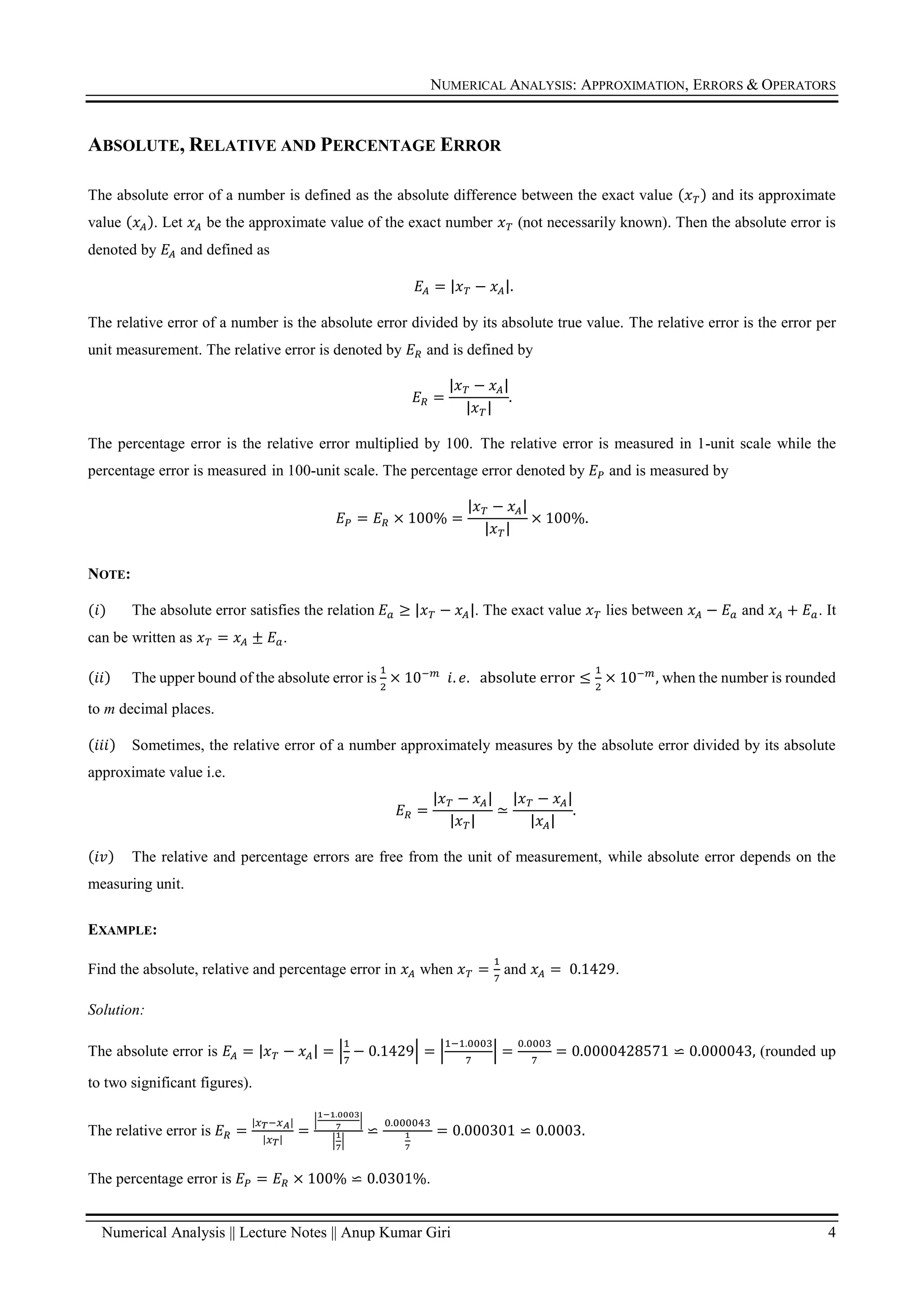
ABSOLUTE, RELATIVE AND PERCENTAGE ERROR
The absolute error of a number is defined as the absolute difference between the exact value (𝑥𝑇) and its approximate
value (𝑥𝐴). Let 𝑥𝐴 be the approximate value of the exact number 𝑥𝑇 (not necessarily known). Then the absolute error is
denoted by 𝐸𝐴 and defined as
𝐸𝐴 = |𝑥𝑇 − 𝑥𝐴|.
The relative error of a number is the absolute error divided by its absolute true value. The relative error is the error per
unit measurement. The relative error is denoted by 𝐸𝑅 and is defined by
𝐸𝑅 =
|𝑥𝑇 − 𝑥𝐴|
|𝑥𝑇|
.
The percentage error is the relative error multiplied by 100. The relative error is measured in 1-unit scale while the
percentage error is measured in 100-unit scale. The percentage error denoted by 𝐸𝑃 and is measured by
𝐸𝑃 = 𝐸𝑅 × 100% =
|𝑥𝑇 − 𝑥𝐴|
|𝑥𝑇|
× 100%.
NOTE:
(𝑖) The absolute error satisfies the relation 𝐸𝑎 ≥ |𝑥𝑇 − 𝑥𝐴|. The exact value 𝑥𝑇 lies between 𝑥𝐴 − 𝐸𝑎 and 𝑥𝐴 + 𝐸𝑎. It
can be written as 𝑥𝑇 = 𝑥𝐴 ± 𝐸𝑎.
(𝑖𝑖) The upper bound of the absolute error is
1
2
× 10−𝑚
𝑖. 𝑒. absolute error ≤
1
2
× 10−𝑚
, when the number is rounded
to m decimal places.
(𝑖𝑖𝑖) Sometimes, the relative error of a number approximately measures by the absolute error divided by its absolute
approximate value i.e.
𝐸𝑅 =
|𝑥𝑇 − 𝑥𝐴|
|𝑥𝑇|
≃
|𝑥𝑇 − 𝑥𝐴|
|𝑥𝐴|
.
(𝑖𝑣) The relative and percentage errors are free from the unit of measurement, while absolute error depends on the
measuring unit.
EXAMPLE:
Find the absolute, relative and percentage error in 𝑥𝐴 when 𝑥𝑇 =
1
7
and 𝑥𝐴 = 0.1429.
Solution:
The absolute error is 𝐸𝐴 = |𝑥𝑇 − 𝑥𝐴| = |
1
7
− 0.1429| = |
1−1.0003
7
| =
0.0003
7
= 0.0000428571 ⋍ 0.000043, (rounded up
to two significant figures).
The relative error is 𝐸𝑅 =
|𝑥𝑇−𝑥𝐴|
|𝑥𝑇|
=
|
1−1.0003
7
|
|
1
7
|
⋍
0.000043
1
7
= 0.000301 ⋍ 0.0003.
The percentage error is 𝐸𝑃 = 𝐸𝑅 × 100% ⋍ 0.0301%.
6.
NUMERICAL ANALYSIS: APPROXIMATION,ERRORS & OPERATORS
Numerical Analysis || Lecture Notes || Anup Kumar Giri 5
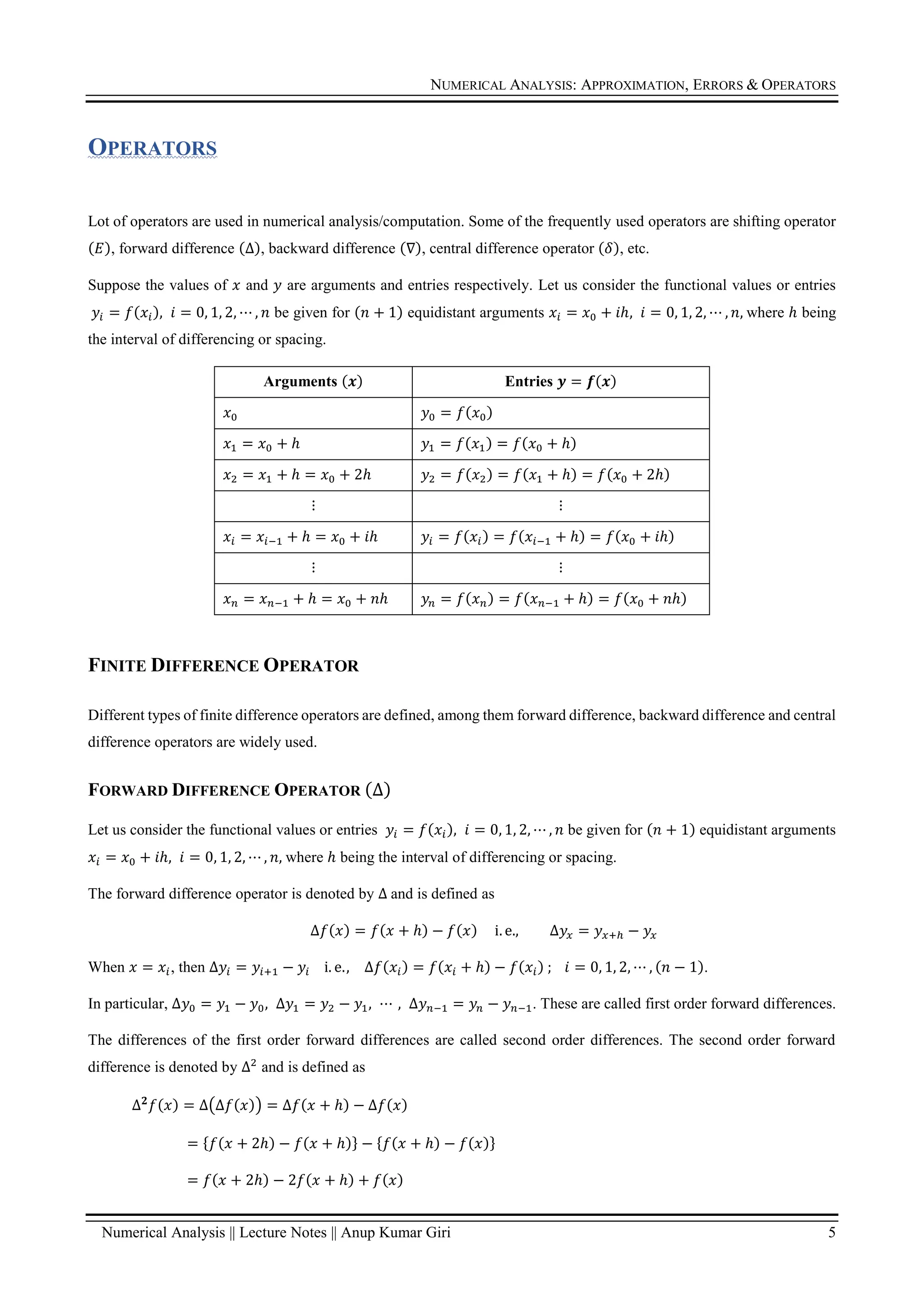
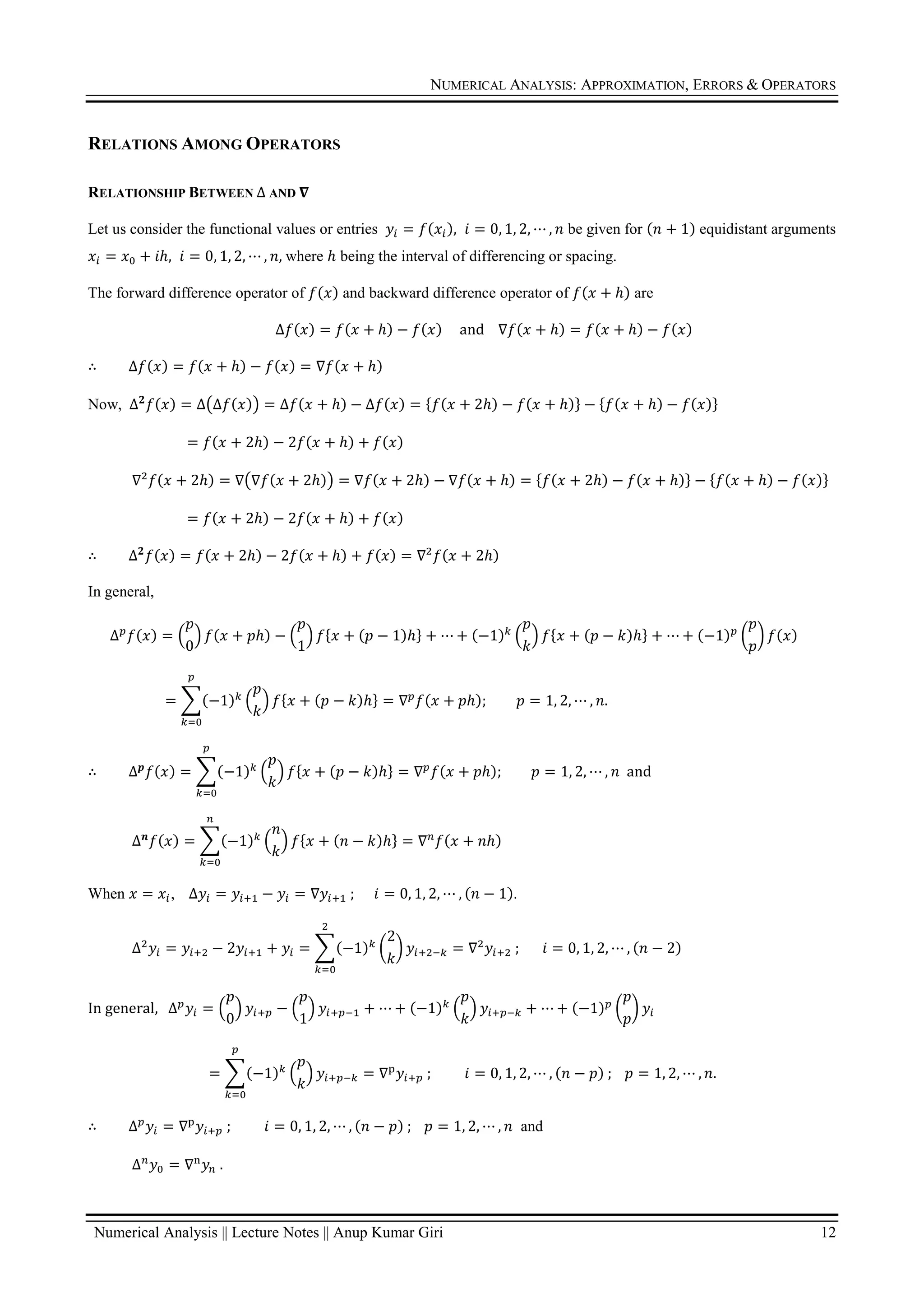
OPERATORS
Lot of operators are used in numerical analysis/computation. Some of the frequently used operators are shifting operator
(𝐸), forward difference (∆), backward difference (∇), central difference operator (𝛿), etc.
Suppose the values of 𝑥 and 𝑦 are arguments and entries respectively. Let us consider the functional values or entries
𝑦𝑖 = 𝑓(𝑥𝑖), 𝑖 = 0, 1, 2, ⋯ , 𝑛 be given for (𝑛 + 1) equidistant arguments 𝑥𝑖 = 𝑥0 + 𝑖ℎ, 𝑖 = 0, 1, 2, ⋯ , 𝑛, where ℎ being
the interval of differencing or spacing.
Arguments (𝒙) Entries 𝒚 = 𝒇(𝒙)
𝑥0 𝑦0 = 𝑓(𝑥0)
𝑥1 = 𝑥0 + ℎ 𝑦1 = 𝑓(𝑥1) = 𝑓(𝑥0 + ℎ)
𝑥2 = 𝑥1 + ℎ = 𝑥0 + 2ℎ 𝑦2 = 𝑓(𝑥2) = 𝑓(𝑥1 + ℎ) = 𝑓(𝑥0 + 2ℎ)
⋮ ⋮
𝑥𝑖 = 𝑥𝑖−1 + ℎ = 𝑥0 + 𝑖ℎ 𝑦𝑖 = 𝑓(𝑥𝑖) = 𝑓(𝑥𝑖−1 + ℎ) = 𝑓(𝑥0 + 𝑖ℎ)
⋮ ⋮
𝑥𝑛 = 𝑥𝑛−1 + ℎ = 𝑥0 + 𝑛ℎ 𝑦𝑛 = 𝑓(𝑥𝑛) = 𝑓(𝑥𝑛−1 + ℎ) = 𝑓(𝑥0 + 𝑛ℎ)
FINITE DIFFERENCE OPERATOR
Different types of finite difference operators are defined, among them forward difference, backward difference and central
difference operators are widely used.
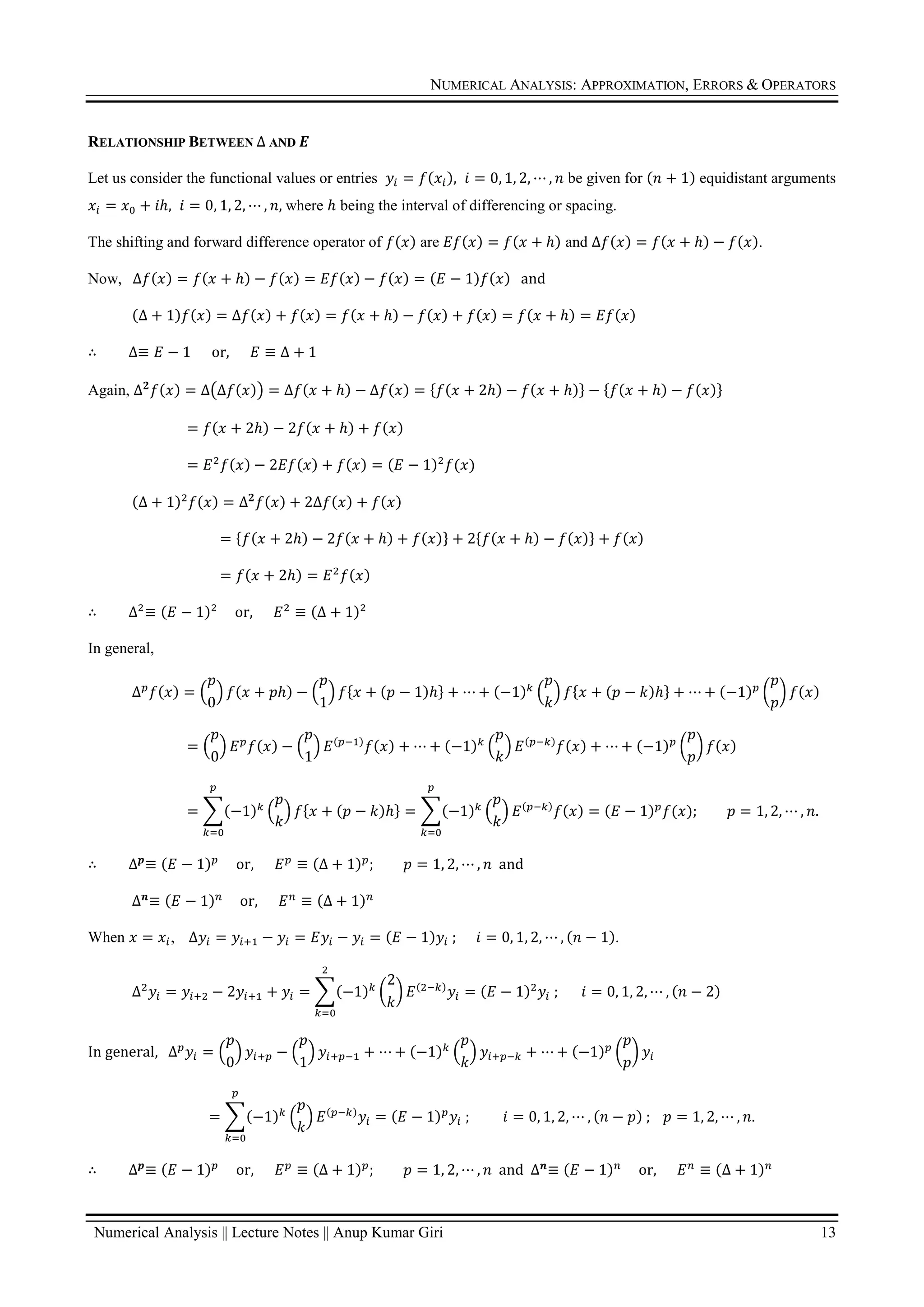
FORWARD DIFFERENCE OPERATOR (∆)
Let us consider the functional values or entries 𝑦𝑖 = 𝑓(𝑥𝑖), 𝑖 = 0, 1, 2, ⋯ , 𝑛 be given for (𝑛 + 1) equidistant arguments
𝑥𝑖 = 𝑥0 + 𝑖ℎ, 𝑖 = 0, 1, 2, ⋯ , 𝑛, where ℎ being the interval of differencing or spacing.
The forward difference operator is denoted by ∆ and is defined as
∆𝑓(𝑥) = 𝑓(𝑥 + ℎ) − 𝑓(𝑥) i. e., ∆𝑦𝑥 = 𝑦𝑥+ℎ − 𝑦𝑥
When 𝑥 = 𝑥𝑖, then ∆𝑦𝑖 = 𝑦𝑖+1 − 𝑦𝑖 i. e., ∆𝑓(𝑥𝑖) = 𝑓(𝑥𝑖 + ℎ) − 𝑓(𝑥𝑖) ; 𝑖 = 0, 1, 2, ⋯ , (𝑛 − 1).
In particular, ∆𝑦0 = 𝑦1 − 𝑦0, ∆𝑦1 = 𝑦2 − 𝑦1, ⋯ , ∆𝑦𝑛−1 = 𝑦𝑛 − 𝑦𝑛−1. These are called first order forward differences.
The differences of the first order forward differences are called second order differences. The second order forward
difference is denoted by ∆2
and is defined as
∆𝟐
𝑓(𝑥) = ∆(∆𝑓(𝑥)) = ∆𝑓(𝑥 + ℎ) − ∆𝑓(𝑥)
= {𝑓(𝑥 + 2ℎ) − 𝑓(𝑥 + ℎ)} − {𝑓(𝑥 + ℎ) − 𝑓(𝑥)}
= 𝑓(𝑥 + 2ℎ) − 2𝑓(𝑥 + ℎ) + 𝑓(𝑥)
NUMERICAL ANALYSIS: APPROXIMATION,ERRORS & OPERATORS
Numerical Analysis || Lecture Notes || Anup Kumar Giri 8
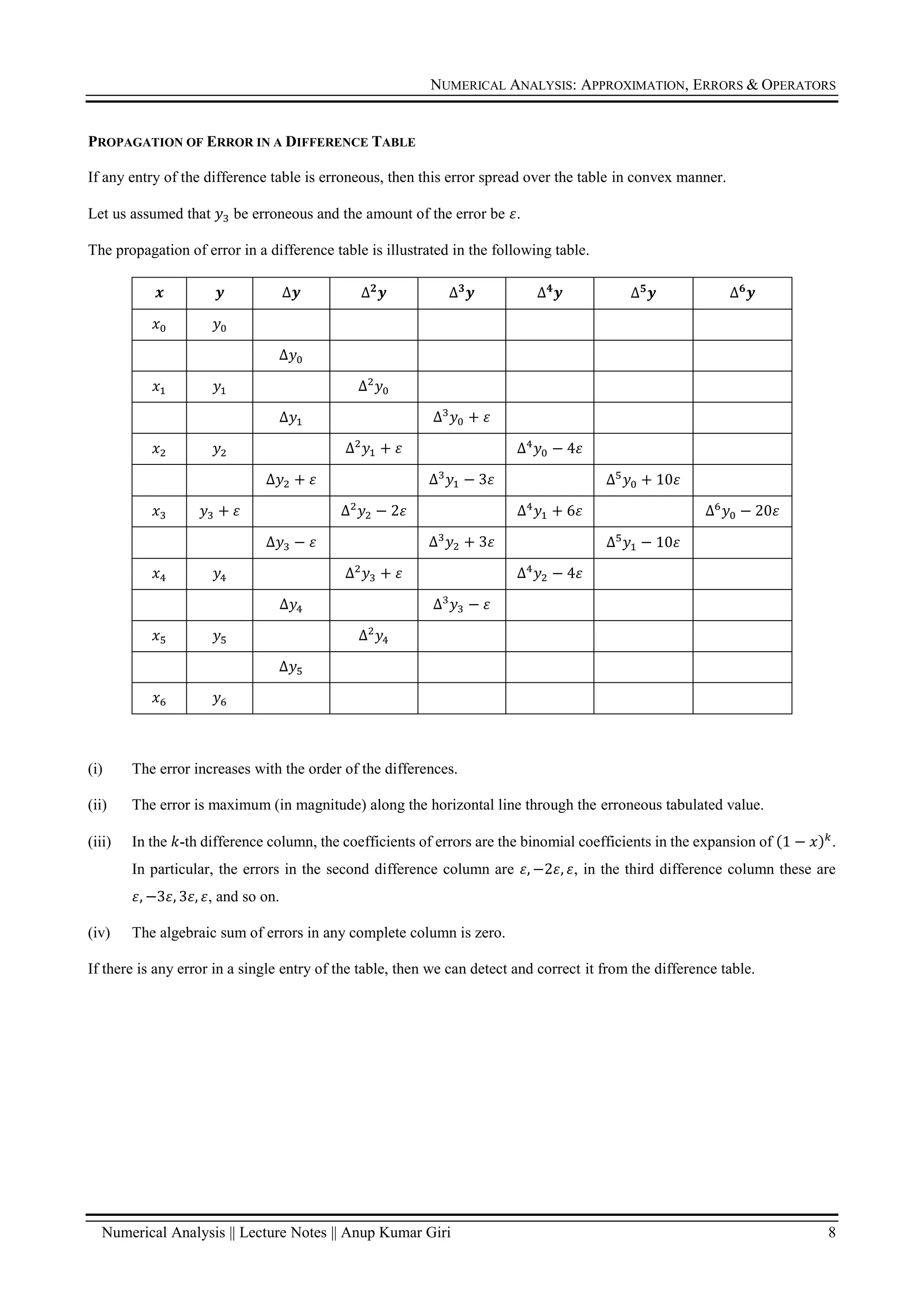
PROPAGATION OF ERROR IN A DIFFERENCE TABLE
If any entry of the difference table is erroneous, then this error spread over the table in convex manner.
Let us assumed that 𝑦3 be erroneous and the amount of the error be 𝜀.
The propagation of error in a difference table is illustrated in the following table.
𝒙 𝒚 ∆𝒚 ∆𝟐
𝒚 ∆𝟑
𝒚 ∆𝟒
𝒚 ∆𝟓
𝒚 ∆𝟔
𝒚
𝑥0 𝑦0
∆𝑦0
𝑥1 𝑦1 ∆2
𝑦0
∆𝑦1 ∆3
𝑦0 + 𝜀
𝑥2 𝑦2 ∆2
𝑦1 + 𝜀 ∆4
𝑦0 − 4𝜀
∆𝑦2 + 𝜀 ∆3
𝑦1 − 3𝜀 ∆5
𝑦0 + 10𝜀
𝑥3 𝑦3 + 𝜀 ∆2
𝑦2 − 2𝜀 ∆4
𝑦1 + 6𝜀 ∆6
𝑦0 − 20𝜀
∆𝑦3 − 𝜀 ∆3
𝑦2 + 3𝜀 ∆5
𝑦1 − 10𝜀
𝑥4 𝑦4 ∆2
𝑦3 + 𝜀 ∆4
𝑦2 − 4𝜀
∆𝑦4 ∆3
𝑦3 − 𝜀
𝑥5 𝑦5 ∆2
𝑦4
∆𝑦5
𝑥6 𝑦6
(i) The error increases with the order of the differences.
(ii) The error is maximum (in magnitude) along the horizontal line through the erroneous tabulated value.
(iii) In the 𝑘-th difference column, the coefficients of errors are the binomial coefficients in the expansion of (1 − 𝑥)𝑘
.
In particular, the errors in the second difference column are 𝜀, −2𝜀, 𝜀, in the third difference column these are
𝜀, −3𝜀, 3𝜀, 𝜀, and so on.
(iv) The algebraic sum of errors in any complete column is zero.
If there is any error in a single entry of the table, then we can detect and correct it from the difference table.
10.
NUMERICAL ANALYSIS: APPROXIMATION,ERRORS & OPERATORS
Numerical Analysis || Lecture Notes || Anup Kumar Giri 9
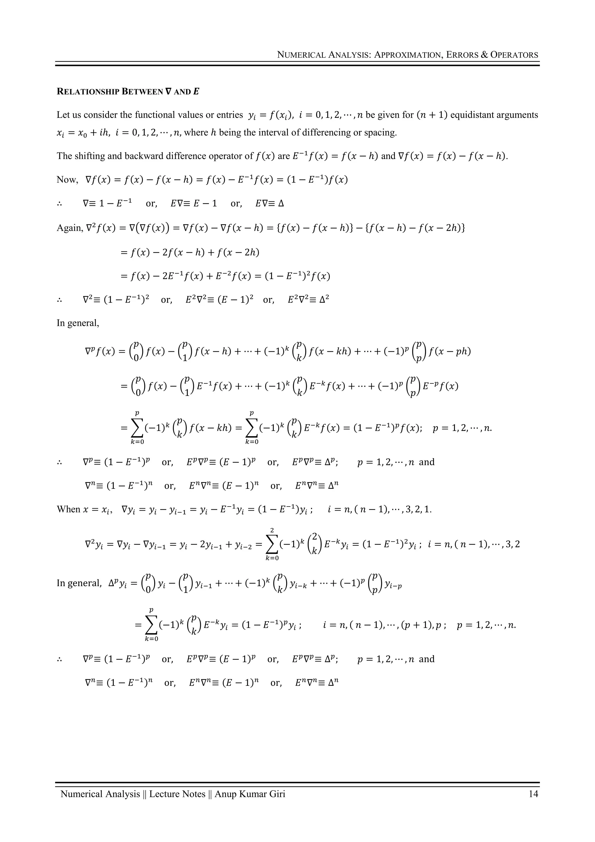
BACKWARD DIFFERENCE OPERATOR (𝛁)
Let us consider the functional values or entries 𝑦𝑖 = 𝑓(𝑥𝑖), 𝑖 = 0, 1, 2, ⋯ , 𝑛 be given for (𝑛 + 1) equidistant arguments
𝑥𝑖 = 𝑥0 + 𝑖ℎ, 𝑖 = 0, 1, 2, ⋯ , 𝑛, where ℎ being the interval of differencing or spacing.
The backward difference operator is denoted by ∇ and is defined as
∇𝑓(𝑥) = 𝑓(𝑥) − 𝑓(𝑥 − ℎ) i. e., ∇𝑦𝑥 = 𝑦𝑥 − 𝑦𝑥−ℎ
When 𝑥 = 𝑥𝑖, then ∇𝑦𝑖 = 𝑦𝑖 − 𝑦𝑖−1 i. e., ∇𝑓(𝑥𝑖) = 𝑓(𝑥𝑖) − 𝑓(𝑥𝑖 − ℎ) ; 𝑖 = 𝑛, ( 𝑛 − 1), ⋯ , 3, 2, 1.
In particular, ∇𝑦1 = 𝑦1 − 𝑦0, ∇𝑦2 = 𝑦2 − 𝑦1, ⋯ , ∇𝑦𝑛 = 𝑦𝑛 − 𝑦𝑛−1. These are called first order backward differences.
The differences of the first order backward differences are called second order backward differences. The second order
backward difference is denoted by ∇2
and is defined as
∇2
𝑓(𝑥) = ∇(∇𝑓(𝑥)) = ∇𝑓(𝑥) − ∇𝑓(𝑥 − ℎ) = {𝑓(𝑥) − 𝑓(𝑥 − ℎ)} − {𝑓(𝑥 − ℎ) − 𝑓(𝑥 − 2ℎ)}
= 𝑓(𝑥) − 2𝑓(𝑥 − ℎ) + 𝑓(𝑥 − 2ℎ)
The second order backward differences are
∇2
𝑦𝑖 = ∇(∇𝑦𝑖) = ∇𝑦𝑖 − ∇𝑦𝑖−1 = 𝑦𝑖 − 2𝑦𝑖−1 + 𝑦𝑖−2 = ∑(−1)𝑘
(
2
𝑘
) 𝑦𝑖−𝑘
2
𝑘=0
; 𝑖 = 𝑛, ( 𝑛 − 1), ⋯ , 3, 2.
The third order backward differences are also defined in similar manner, i.e.,
∇3
𝑦𝑖 = ∇(∇2
𝑦𝑖) = ∇2
𝑦𝑖 − ∇2
𝑦𝑖−1 = (𝑦𝑖 − 2𝑦𝑖−1 + 𝑦𝑖−2) − (𝑦𝑖−1 − 2𝑦𝑖−2 + 𝑦𝑖−3)
= 𝑦𝑖 − 3𝑦𝑖−1 + 3𝑦𝑖−2 − 𝑦𝑖−3 = ∑(−1)𝑘
(
3
𝑘
) 𝑦𝑖−𝑘
3
𝑘=0
; 𝑖 = 𝑛, ( 𝑛 − 1), ⋯ , 4, 3.
Similarly, higher order differences can be defined.
In general,
∇𝑝
𝑦𝑖 = ∇(∇𝑝−1
𝑦𝑖) = ∇𝑝−1
𝑦𝑖 − ∇𝑝−1
𝑦𝑖−1 or, [∇𝑝
𝑦𝑖 = ∇𝑝−1(∆𝑦𝑖)]
= (
𝑝
0
) 𝑦𝑖 − (
𝑝
1
) 𝑦𝑖−1 + ⋯ + (−1)𝑘
(
𝑝
𝑘
) 𝑦𝑖−𝑘 + ⋯ + (−1)𝑝−1
(
𝑝
𝑝 − 1
) 𝑦𝑖−𝑝+1 + (−1)𝑝
(
𝑝
𝑝
) 𝑦𝑖−𝑝
= ∑(−1)𝑘
(
𝑝
𝑘
) 𝑦𝑖−𝑘
𝑝
𝑘=0
; 𝑖 = 𝑛, ( 𝑛 − 1), ⋯ , (𝑝 + 1), 𝑝 ; 𝑝 = 1, 2, ⋯ , 𝑛.
We may write
∇𝑛
𝑦𝑛 = (
𝑛
0
) 𝑦𝑛 − (
𝑛
1
) 𝑦𝑛−1 + ⋯ + (−1)𝑘
(
𝑛
𝑘
) 𝑦𝑛−𝑘 + ⋯ + (−1)𝑛
(
𝑛
𝑛
) 𝑦0 = ∑(−1)𝑘
(
𝑛
𝑘
) 𝑦𝑛−𝑘
𝑛
𝑘=0
NOTE:
∇0
𝑓(𝑥) = 𝑓(𝑥) and ∇𝑝
𝑓(𝑥) = 0 for all 𝑝 > 𝑛.
11.
NUMERICAL ANALYSIS: APPROXIMATION,ERRORS & OPERATORS
Numerical Analysis || Lecture Notes || Anup Kumar Giri 10
BACKWARD DIFFERENCE TABLE
Backward differences can be represented in a tabular form, called the backward difference or horizontal difference table.
𝒙 𝒚 = 𝒇(𝒙) 𝛁𝒚 𝛁𝟐
𝒚 𝛁𝟑
𝒚
𝑥0 𝑦0 = 𝑓(𝑥0)
𝑥1 = 𝑥0 + ℎ 𝑦1 = 𝑓(𝑥1) ∇𝑦1 = 𝑦1 − 𝑦0
𝑥2 = 𝑥0 + 2ℎ 𝑦2 = 𝑓(𝑥2) ∇𝑦2 = 𝑦2 − 𝑦1 ∇2
𝑦2 = ∇𝑦2 − ∇𝑦1
𝑥3 = 𝑥0 + 3ℎ 𝑦3 = 𝑓(𝑥3) ∇𝑦3 = 𝑦3 − 𝑦2 ∇2
𝑦3 = ∇𝑦3 − ∇𝑦2 ∇3
𝑦3 = ∇2
𝑦3 − ∇2
𝑦2
It is observed from the forward and backward difference tables that for a given table of values both the tables are same.
Practically, there are no differences among the values of the tables, but theoretically they have separate significant.
SHIFTING OPERATOR (𝑬)
Let us consider the functional values or entries 𝑦𝑖 = 𝑓(𝑥𝑖), 𝑖 = 0, 1, 2, ⋯ , 𝑛 be given for (𝑛 + 1) equidistant arguments
𝑥𝑖 = 𝑥0 + 𝑖ℎ, 𝑖 = 0, 1, 2, ⋯ , 𝑛, where ℎ being the interval of differencing or spacing.
The shifting operator is denoted by 𝐸 and is defined as
𝐸𝑓(𝑥) = 𝑓(𝑥 + ℎ)
When 𝑥 = 𝑥𝑖, 𝐸𝑓(𝑥𝑖) = 𝑓(𝑥𝑖 + ℎ) or, 𝐸(𝑦𝑖) = 𝑦𝑖+1 ; 𝑖 = 0, 1, 2, ⋯ , (𝑛 − 1).
Now, 𝐸2
𝑓(𝑥) = 𝐸{𝐸𝑓(𝑥)} = 𝐸{𝑓(𝑥 + ℎ)} = 𝑓(𝑥 + 2ℎ) or, 𝐸2(𝑦𝑖) = 𝑦𝑖+2 ; 𝑖 = 0, 1, 2, ⋯ , (𝑛 − 2).
In general,
𝐸𝑝
𝑓(𝑥) = 𝐸𝑝−1[𝐸𝑓(𝑥)] = 𝐸𝑝−1[𝑓(𝑥 + ℎ)] = ⋯ = 𝐸𝑝−𝑘[𝑓(𝑥 + 𝑘ℎ)] = ⋯ = 𝐸𝑓[𝑥 + (𝑝 − 1)ℎ] = 𝑓(𝑥 + 𝑝ℎ)
i. e., 𝐸𝑝(𝑦𝑖) = 𝑦𝑖+𝑝 ; 𝑖 = 0, 1, 2, ⋯ , (𝑛 − 𝑝); 𝑝 = 1, 2, ⋯ , 𝑛.
We may write 𝐸𝑛
𝑓(𝑥) = 𝑓(𝑥 + 𝑛ℎ) or, 𝐸𝑛(𝑦0) = 𝑦𝑛.
The inverse shifting operator denoted by 𝐸−1
and is defined as
𝐸−1
𝑓(𝑥) = 𝑓(𝑥 − ℎ).
When 𝑥 = 𝑥𝑖, 𝐸−1
𝑓(𝑥𝑖) = 𝑓(𝑥𝑖 − ℎ) or, 𝐸−1(𝑦𝑖) = 𝑦𝑖−1 ; 𝑖 = 𝑛, ( 𝑛 − 1), ⋯ , 3, 2, 1.
Now, 𝐸−2
𝑓(𝑥) = 𝐸−1{𝐸−1
𝑓(𝑥)} = 𝐸−1{𝑓(𝑥 − ℎ)} = 𝑓(𝑥 − 2ℎ) or, 𝐸−2(𝑦𝑖) = 𝑦𝑖−2 ; 𝑖 = 𝑛, ( 𝑛 − 1), ⋯ , 3, 2.
In general,
𝐸−𝑝
𝑓(𝑥) = 𝐸−(𝑝−1)[𝑓(𝑥 − ℎ)] = ⋯ = 𝐸−(𝑝−𝑘)[𝑓(𝑥 − 𝑘ℎ)] = ⋯ = 𝐸−1
𝑓{𝑥 − (𝑝 − 1)ℎ} = 𝑓(𝑥 − 𝑝ℎ)
i. e., 𝐸−𝑝(𝑦𝑖) = 𝑦𝑖−𝑝 ; 𝑖 = 𝑛, ( 𝑛 − 1), ⋯ , (𝑝 + 1), 𝑝 ; 𝑝 = 1, 2, ⋯ , 𝑛.
We may write 𝐸−𝑛
𝑓(𝑥) = 𝑓(𝑥 − 𝑛ℎ) or, 𝐸−𝑛(𝑦𝑛) = 𝑦0.
NUMERICAL ANALYSIS: APPROXIMATION,ERRORS & OPERATORS
Numerical Analysis || Lecture Notes || Anup Kumar Giri 16
Similarly,
∆2
𝑓(𝑥) = 𝑎𝑛−1
(1)
[(𝑥 + ℎ)𝑛−1
− 𝑥𝑛−1] + 𝑎𝑛−2
(1)
[(𝑥 + ℎ)𝑛−2
− 𝑥𝑛−2] + ⋯ + 𝑎2
(1)
[(𝑥 + ℎ)2
− 𝑥2] + 𝑎1
(1)
[(𝑥 + ℎ) − 𝑥]
= 𝑎𝑛−2
(2)
𝑥𝑛−2
+ 𝑎𝑛−3
(2)
𝑥𝑛−3
+ ⋯ + 𝑎2
(2)
𝑥2
+ 𝑎1
(2)
𝑥 + 𝑎0
(2)
The coefficients 𝑎𝑖
(2)
's, 𝑖 = 1, 2, ⋯ , (𝑛 − 2) are suitable constants and 𝑎𝑛−2
(2)
= 𝑎𝑛−1
(1)
(𝑛 − 1)ℎ = 𝑎𝑛{𝑛(𝑛 − 1)}ℎ2
.
The second difference of a polynomial of the 𝑛-th degree is thus another polynomial of degree (𝑛 − 2).
In general, ∆𝑝
𝑓(𝑥) = 𝑎𝑛−𝑝+1
(𝑝−1)
[(𝑥 + ℎ)𝑛−𝑝+1
− 𝑥𝑛−𝑝+1] + ⋯ + 𝑎2
(𝑝−1)
[(𝑥 + ℎ)2
− 𝑥2] + 𝑎1
(𝑝−1)
[(𝑥 + ℎ) − 𝑥]
= 𝑎𝑛−𝑝
(𝑝)
𝑥𝑛−𝑝
+ 𝑎𝑛−𝑝−1
(𝑝)
𝑥𝑛−3
+ ⋯ + 𝑎2
(𝑝)
𝑥2
+ 𝑎1
(𝑝)
𝑥 + 𝑎0
(𝑝)
The coefficients 𝑎𝑖
(𝑝)
's, 𝑖 = 1, 2, ⋯ , (𝑛 − 𝑝) are suitable constants and
𝑎𝑛−𝑝
(𝑝)
= 𝑎𝑛−𝑝+1
(𝑝−1)
(𝑛 − 𝑝 + 1)ℎ = 𝑎𝑛{𝑛(𝑛 − 1) ⋯ (𝑛 − 𝑝 + 1)}ℎ𝑝
.
The 𝑝-th difference of a polynomial of the 𝑛-th degree is thus another polynomial of degree (𝑛 − 𝑝).
In this manner we arrive at a polynomial of zero degree for the 𝑛-th difference; that is,
∆𝑛
𝑓(𝑥) = 𝑎0
(𝑛)
= 𝑎1
(𝑛−1)
∙ 1 ∙ ℎ = 𝑎𝑛{𝑛(𝑛 − 1) ⋯ 3 ∙ 2 ∙ 1}ℎ𝑛
= 𝑎𝑛𝑛! ℎ𝑛
The 𝑛-th difference is therefore constant, and all higher differences are zero.
Hence, ∆𝑝
𝑓(𝑥), 𝑝 < 𝑛 is a polynomial of degree (𝑛 − 𝑝),
∆𝑛
𝑓(𝑥) = 𝑎𝑛{𝑛(𝑛 − 1) ⋯ 3 ∙ 2 ∙ 1}ℎ𝑛
= 𝑎𝑛𝑛! ℎ𝑛
= constant, and
∆𝑝
𝑓(𝑥) = 0 if 𝑝 > 𝑛.
NOTE:
The 𝑛-th differences of a polynomial of the 𝑛-th degree are constant when the values of the independent variable are taken
in arithmetic progression or with equal interval of differencing.
The converse of this proposition is also true, that is, if the 𝑛-th differences of a tabulated function are constant when the
values of the independent variable are taken in arithmetic progression, the function is a polynomial of degree 𝑛.
18.
NUMERICAL ANALYSIS: APPROXIMATION,ERRORS & OPERATORS
Numerical Analysis || Lecture Notes || Anup Kumar Giri 17
BACKWARD DIFFERENCE OF A POLYNOMIAL
Let 𝑓(𝑥) = 𝑎𝑛𝑥𝑛
+ 𝑎𝑛−1𝑥𝑛−1
+ ⋯ + 𝑎2𝑥2
+ 𝑎1𝑥 + 𝑎0 (𝑎𝑛 ≠ 0) be a polynomial in 𝑥 of degree 𝑛, where 𝑎𝑖's be the
given coefficients. Let us consider ℎ be the interval of differencing.
Now, ∇𝑓(𝑥) = 𝑓(𝑥) − 𝑓(𝑥 − ℎ)
= 𝑎𝑛[𝑥𝑛
− (𝑥 − ℎ)𝑛] + 𝑎𝑛−1[𝑥𝑛−1
− (𝑥 − ℎ)𝑛−1] + ⋯ + 𝑎2[𝑥2
− (𝑥 − ℎ)2] + 𝑎1[𝑥 − (𝑥 − ℎ)]
= 𝑎𝑛 [𝑥𝑛
− 𝑥𝑛
+ (
𝑛
1
) 𝑥𝑛−1
ℎ − (
𝑛
2
) 𝑥𝑛−2
ℎ2
+ ⋯ + (−1)𝑛
(
𝑛
𝑛 − 1
) 𝑥ℎ𝑛−1
+ (−1)𝑛+1
(
𝑛
𝑛
) ℎ𝑛
]
+ 𝑎𝑛−1 [𝑥𝑛−1
− 𝑥𝑛−1
+ (
𝑛 − 1
1
) 𝑥𝑛−2
ℎ + ⋯ + (−1)𝑛−1
(
𝑛 − 1
𝑛 − 2
) 𝑥ℎ𝑛−2
+ (−1)𝑛
ℎ𝑛−1
] + ⋯
+ 𝑎2 [𝑥2
− 𝑥2
+ (
2
1
) 𝑥ℎ − ℎ2
] + 𝑎1ℎ
= 𝑎𝑛𝑛ℎ𝑥𝑛−1
+ [−𝑎𝑛 (
𝑛
2
) ℎ2
+ 𝑎𝑛−1 (
𝑛 − 1
1
) ℎ] 𝑥𝑛−2
+ ⋯
+ [𝑎𝑛(−1)𝑛
(
𝑛
𝑛 − 1
) ℎ𝑛−1
+ 𝑎𝑛−1(−1)𝑛−1
(
𝑛 − 1
𝑛 − 2
) ℎ𝑛−2
+ ⋯ + 𝑎2(−1)2−1
(
2
1
) ℎ] 𝑥
+ [𝑎𝑛(−1)𝑛+1
ℎ𝑛
+ 𝑎𝑛−1(−1)𝑛
ℎ𝑛−1
+ ⋯ − 𝑎2ℎ2
+ 𝑎1ℎ]
= 𝑎𝑛−1
(1)
𝑥𝑛−1
+ 𝑎𝑛−2
(1)
𝑥𝑛−2
+ ⋯ + 𝑎2
(1)
𝑥2
+ 𝑎1
(1)
𝑥 + 𝑎0
(1)
The coefficients 𝑎𝑖
(1)
's are suitable constants and 𝑎𝑛−1
(1)
= 𝑎𝑛𝑛ℎ.
The first backward difference of a polynomial of the 𝑛-th degree is thus another polynomial of degree (𝑛 − 1).
Similarly,
∇2
𝑓(𝑥) = 𝑎𝑛−1
(1)
[𝑥𝑛−1
− (𝑥 − ℎ)𝑛−1] + 𝑎𝑛−2
(1)
[𝑥𝑛−2
− (𝑥 − ℎ)𝑛−2] + ⋯ + 𝑎2
(1)
[𝑥2
− (𝑥 − ℎ)2] + 𝑎1
(1)
[𝑥 − (𝑥 − ℎ)]
= 𝑎𝑛−2
(2)
𝑥𝑛−2
+ 𝑎𝑛−3
(2)
𝑥𝑛−3
+ ⋯ + 𝑎2
(2)
𝑥2
+ 𝑎1
(2)
𝑥 + 𝑎0
(2)
The coefficients 𝑎𝑖
(2)
's are suitable constants and 𝑎𝑛−2
(2)
= 𝑎𝑛−1
(1)
(𝑛 − 1)ℎ = 𝑎𝑛{𝑛(𝑛 − 1)}ℎ2
.
The second backward difference of a polynomial of the 𝑛-th degree is thus another polynomial of degree (𝑛 − 2).
In general, ∇𝑝
𝑓(𝑥) = 𝑎𝑛−𝑝+1
(𝑝−1)
[𝑥𝑛−𝑝+1
− (𝑥 − ℎ)𝑛−𝑝+1] + ⋯ + 𝑎2
(𝑝−1)
[𝑥2
− (𝑥 − ℎ)2] + 𝑎1
(𝑝−1)
[𝑥 − (𝑥 − ℎ)]
= 𝑎𝑛−𝑝
(𝑝)
𝑥𝑛−𝑝
+ 𝑎𝑛−𝑝−1
(𝑝)
𝑥𝑛−3
+ ⋯ + 𝑎2
(𝑝)
𝑥2
+ 𝑎1
(𝑝)
𝑥 + 𝑎0
(𝑝)
The coefficients 𝑎𝑖
(𝑝)
's are suitable constants and
𝑎𝑛−𝑝
(𝑝)
= 𝑎𝑛−𝑝+1
(𝑝−1)
(𝑛 − 𝑝 + 1)ℎ = 𝑎𝑛{𝑛(𝑛 − 1) ⋯ (𝑛 − 𝑝 + 1)}ℎ𝑝
.
The 𝑝-th backward difference of a polynomial of the 𝑛-th degree is thus another polynomial of degree (𝑛 − 𝑝).
In this manner we arrive at a polynomial of zero degree for the 𝑛-th backward difference; that is,
∇𝑛
𝑓(𝑥) = 𝑎0
(𝑛)
= 𝑎1
(𝑛−1)
∙ 1 ∙ ℎ = 𝑎𝑛{𝑛(𝑛 − 1) ⋯ 3 ∙ 2 ∙ 1}ℎ𝑛
= 𝑎𝑛𝑛! ℎ𝑛
The 𝑛-th backward difference is therefore constant, and all higher backward differences are zero.
19.
NUMERICAL ANALYSIS: APPROXIMATION,ERRORS & OPERATORS
Numerical Analysis || Lecture Notes || Anup Kumar Giri 18
Hence, ∇𝑝
𝑓(𝑥), 𝑝 < 𝑛 is a polynomial of degree (𝑛 − 𝑝),
∇𝑛
𝑓(𝑥) = 𝑎𝑛{𝑛(𝑛 − 1) ⋯ 3 ∙ 2 ∙ 1}ℎ𝑛
= 𝑎𝑛𝑛! ℎ𝑛
= constant, and
∇𝑝
𝑓(𝑥) = 0 if 𝑝 > 𝑛.
NOTE:
The 𝑛-th backward differences of a polynomial of the 𝑛-th degree are constant when the values of the independent variable
are taken in arithmetic progression or with equal interval of differencing.
The converse of this proposition is also true, that is, if the 𝑛-th backward differences of a tabulated function are constant
when the values of the independent variable are taken in arithmetic progression, the function is a polynomial of degree 𝑛.
PROBLEM
Show that 𝐸∆≡ ∆𝐸 and ∆∇≡ ∇∆.
Solution:
𝐸∆𝑓(𝑥) = 𝐸[∆𝑓(𝑥)] = 𝐸[𝑓(𝑥 + ℎ) − 𝑓(𝑥)] = 𝐸𝑓(𝑥 + ℎ) − 𝐸𝑓(𝑥) = 𝑓(𝑥 + 2ℎ) − 𝑓(𝑥 + ℎ) = ∆𝑓(𝑥 + ℎ) = ∆𝐸𝑓(𝑥)
∆∇𝑓(𝑥) = ∆[𝑓(𝑥) − 𝑓(𝑥 − ℎ)] = ∆𝑓(𝑥) − ∆𝑓(𝑥 − ℎ)
= [𝑓(𝑥 + ℎ) − 𝑓(𝑥)] − [𝑓(𝑥) − 𝑓(𝑥 − ℎ)]
= ∇𝑓(𝑥 + ℎ) − ∇𝑓(𝑥) = ∇[𝑓(𝑥 + ℎ) − 𝑓(𝑥)] = ∇∆𝑓(𝑥)
∴ 𝐸∆≡ ∆𝐸 and ∆∇≡ ∇∆.
PROBLEM
Suppose 𝑈0 = −3, 𝑈1 = 6, 𝑈2 = 8 and 𝑈3 = 12. Find 𝑈6.
Solution:
From the given data, we get the following difference table.
Argument (𝑥) Entry (𝑈𝑥) ∆𝑈𝑥 ∆2
𝑈𝑥 ∆3
𝑈𝑥
0 −3
∆𝑈0 = 9
1 6 ∆2
𝑈0 = −7
∆𝑈1 = 2 ∆3
𝑈0 = 9
2 8 ∆2
𝑈1 = 2
∆𝑈2 = 4
3 12
Since four entries 𝑈𝑥 for the arguments 𝑥 = 0, 1, 2, 3 are given, we may assume that the fourth and higher order forward
differences are zero i.e., ∆𝑘
𝑈0 = 0 ; 𝑘 ≥ 4.
Now, 𝑈6 = 𝐸6
𝑈0 = (∆ + 1)6
𝑈0 = (
6
0
) ∆6
𝑈0 + (
6
1
) ∆5
𝑈0 + (
6
2
) ∆4
𝑈0 + (
6
3
) ∆3
𝑈0 + (
6
4
) ∆2
𝑈0 + (
6
5
) ∆𝑈0 + (
6
6
) 𝑈0
= 20∆3
𝑈0 + 15∆2
𝑈0 + 6∆𝑈0 + 𝑈0 = 20 × 9 + 15 × (−7) + 6 × 9 + (−3) = 126
![NUMERICAL ANALYSIS: APPROXIMATION, ERRORS & OPERATORS
Numerical Analysis || Lecture Notes || Anup Kumar Giri 6
The second order forward differences are
∆2
𝑦𝑖 = ∆(∆𝑦𝑖) = ∆𝑦𝑖+1 − ∆𝑦𝑖 = 𝑦𝑖+2 − 2𝑦𝑖+1 + 𝑦𝑖 = ∑(−1)𝑘
(
2
𝑘
) 𝑦𝑖+2−𝑘
2
𝑘=0
; 𝑖 = 0, 1, 2, ⋯ , (𝑛 − 2)
The third order forward differences are also defined in similar manner, i.e.,
∆3
𝑦𝑖 = ∆(∆2
𝑦𝑖) = ∆2
𝑦𝑖+1 − ∆2
𝑦𝑖 = (𝑦𝑖+3 − 2𝑦𝑖+2 + 𝑦𝑖+1) − (𝑦𝑖+2 − 2𝑦𝑖+1 + 𝑦𝑖)
= 𝑦𝑖+3 − 3𝑦𝑖+2 + 3𝑦𝑖+1 − 𝑦𝑖 = ∑(−1)𝑘
(
3
𝑘
) 𝑦𝑖+3−𝑘
3
𝑘=0
; 𝑖 = 0, 1, 2, ⋯ , (𝑛 − 3)
Similarly, higher order differences can be defined.
In general,
∆𝑝
𝑦𝑖 = ∆(∆𝑝−1
𝑦𝑖) = ∆𝑝−1
𝑦𝑖+1 − ∆𝑝−1
𝑦𝑖 or, [∆𝑝
𝑦𝑖 = ∆𝑝−1(∆𝑦𝑖)]
= (
𝑝
0
) 𝑦𝑖+𝑝 − (
𝑝
1
) 𝑦𝑖+𝑝−1 + ⋯ + (−1)𝑘
(
𝑝
𝑘
) 𝑦𝑖+𝑝−𝑘 + ⋯ + (−1)𝑝−1
(
𝑝
𝑝 − 1
) 𝑦𝑖+1 + (−1)𝑝
(
𝑝
𝑝
) 𝑦𝑖
= ∑(−1)𝑘
(
𝑝
𝑘
) 𝑦𝑖+𝑝−𝑘
𝑝
𝑘=0
; 𝑖 = 0, 1, 2, ⋯ , (𝑛 − 𝑝) ; 𝑝 = 1, 2, ⋯ , 𝑛.
We may write
∆𝑛
𝑦0 = (
𝑛
0
) 𝑦𝑛 − (
𝑛
1
) 𝑦𝑛−1 + ⋯ + (−1)𝑘
(
𝑛
𝑘
) 𝑦𝑛−𝑘 + ⋯ + (−1)𝑛
(
𝑛
𝑛
) 𝑦0 = ∑(−1)𝑘
(
𝑛
𝑘
) 𝑦𝑛−𝑘
𝑛
𝑘=0
NOTE:
∆0
𝑓(𝑥) = 𝑓(𝑥) and ∆𝑝
𝑓(𝑥) = 0 for all 𝑝 > 𝑛.
FINITE / FORWARD DIFFERENCE TABLE
All the forward differences can be represented in a tabular form, called the forward difference or diagonal difference
table.
𝒙 𝒚 = 𝒇(𝒙) ∆𝒚 ∆𝟐
𝒚 ∆𝟑
𝒚
𝑥0 𝑦0 = 𝑓(𝑥0)
∆𝑦0 = 𝑦1 − 𝑦0
𝑥1 = 𝑥0 + ℎ 𝑦1 = 𝑓(𝑥1) ∆2
𝑦0 = ∆𝑦1 − ∆𝑦0
∆𝑦1 = 𝑦2 − 𝑦1 ∆3
𝑦0 = ∆2
𝑦1 − ∆2
𝑦0
𝑥2 = 𝑥0 + 2ℎ 𝑦2 = 𝑓(𝑥2) ∆2
𝑦1 = ∆𝑦2 − ∆𝑦1
∆𝑦2 = 𝑦3 − 𝑦2
𝑥3 = 𝑥0 + 3ℎ 𝑦3 = 𝑓(𝑥3)](https://image.slidesharecdn.com/numericalanalysisapproximationerroroperator-250906012610-5635420b/75/Numerical-Analysis_Approximation-Error-Operator-pdf-7-2048.jpg)
![NUMERICAL ANALYSIS: APPROXIMATION, ERRORS & OPERATORS
Numerical Analysis || Lecture Notes || Anup Kumar Giri 7
PROPERTIES OF ∆
Some common properties of forward difference operator are as follows:
(𝑖) ∆𝑐 = 𝑐 − 𝑐 = 0, where 𝑐 is a constant.
(𝑖𝑖) ∆{𝑐𝑓(𝑥)} = 𝑐𝑓(𝑥 + ℎ) − 𝑐𝑓(𝑥) = 𝑐{𝑓(𝑥 + ℎ) − 𝑓(𝑥)} = 𝑐∆𝑓(𝑥).
(𝑖𝑖𝑖) ∆{𝑓1(𝑥) + 𝑓2(𝑥) + ⋯ + 𝑓𝑚(𝑥)} = {𝑓1(𝑥 + ℎ) + 𝑓2(𝑥 + ℎ) + ⋯ + 𝑓𝑚(𝑥 + ℎ)} − {𝑓1(𝑥) + 𝑓2(𝑥) + ⋯ + 𝑓𝑚(𝑥)}
= ∆𝑓1(𝑥) + ∆𝑓2(𝑥) + ⋯ + ∆𝑓𝑚(𝑥).
(𝑖𝑣) ∆{𝑐1𝑓1(𝑥) + 𝑐2𝑓2(𝑥) + ⋯ + 𝑐𝑚𝑓𝑚(𝑥)} = 𝑐1∆𝑓1(𝑥) + 𝑐2∆𝑓2(𝑥) + ⋯ + 𝑐𝑚∆𝑓𝑚(𝑥).
(𝑣) For any two positive integers 𝑚 and 𝑛,
∆𝑚
∆𝑛
𝑓(𝑥) = ∆𝑚+𝑛
𝑓(𝑥) = ∆𝑛
∆𝑚
𝑓(𝑥) = ∆𝑘
∆𝑚+𝑛−𝑘
𝑓(𝑥) ; 𝑘 = 0, 1, 2, ⋯ , 𝑚 or 𝑛.
(𝑣𝑖) ∆𝑝
𝑓(𝑥𝑖) = (
𝑝
0
) 𝑓(𝑥𝑖 + 𝑝ℎ) − (
𝑝
1
) 𝑓{𝑥𝑖 + (𝑝 − 1)ℎ} + ⋯ + (−1)𝑘
(
𝑝
𝑘
) 𝑓{𝑥𝑖 + (𝑝 − 𝑘)ℎ} + ⋯ + (−1)𝑝
(
𝑝
𝑝
) 𝑓(𝑥𝑖)
= ∑(−1)𝑘
(
𝑝
𝑘
) 𝑓{𝑥𝑖 + (𝑝 − 𝑘)ℎ}
𝑝
𝑘=0
; 𝑖 = 0, 1, 2, ⋯ , (𝑛 − 𝑝), 𝑝 = 1, 2, ⋯ , 𝑛
(𝑣𝑖𝑖) ∆{𝑓(𝑥)𝑔(𝑥)} = 𝑓(𝑥 + ℎ)𝑔(𝑥 + ℎ) − 𝑓(𝑥)𝑔(𝑥)
= 𝑓(𝑥 + ℎ)𝑔(𝑥 + ℎ) − 𝑓(𝑥 + ℎ)𝑔(𝑥) + 𝑓(𝑥 + ℎ)𝑔(𝑥) − 𝑓(𝑥)𝑔(𝑥)
= 𝑓(𝑥 + ℎ){𝑔(𝑥 + ℎ) − 𝑔(𝑥)} + 𝑔(𝑥){𝑓(𝑥 + ℎ) − 𝑓(𝑥)}
= 𝑓(𝑥 + ℎ)∆𝑔(𝑥) + 𝑔(𝑥)∆𝑓(𝑥).
Also, ∆{𝑓(𝑥)𝑔(𝑥)} = 𝑓(𝑥)∆𝑔(𝑥) + 𝑔(𝑥 + ℎ)∆𝑓(𝑥) = 𝑓(𝑥)∆𝑔(𝑥) + 𝑔(𝑥)∆𝑓(𝑥) + ∆𝑓(𝑥)∆𝑔(𝑥).
(𝑣𝑖𝑖𝑖) ∆ {
𝑓(𝑥)
𝑔(𝑥)
} =
𝑔(𝑥)∆𝑓(𝑥) − 𝑓(𝑥)∆𝑔(𝑥)
𝑔(𝑥 + ℎ)𝑔(𝑥)
, 𝑔(𝑥) ≠ 0.
∆ {
𝑓(𝑥)
𝑔(𝑥)
} =
𝑓(𝑥 + ℎ)
𝑔(𝑥 + ℎ)
−
𝑓(𝑥)
𝑔(𝑥)
=
𝑓(𝑥 + ℎ)𝑔(𝑥) − 𝑓(𝑥)𝑔(𝑥 + ℎ)
𝑔(𝑥 + ℎ)𝑔(𝑥)
=
𝑔(𝑥){𝑓(𝑥 + ℎ) − 𝑓(𝑥)} − 𝑓(𝑥){𝑔(𝑥 + ℎ) − 𝑔(𝑥)}
𝑔(𝑥 + ℎ)𝑔(𝑥)
=
𝑔(𝑥)∆𝑓(𝑥) − 𝑓(𝑥)∆𝑔(𝑥)
𝑔(𝑥 + ℎ)𝑔(𝑥)
, 𝑔(𝑥) ≠ 0.
In particular, when the numerator is 1, then
∆ {
1
𝑓(𝑥)
} = −
∆𝑓(𝑥)
𝑓(𝑥 + ℎ)𝑓(𝑥)
, 𝑓(𝑥) ≠ 0 [∵ ∆𝑔(𝑥) = ∆(1) = 0]](https://image.slidesharecdn.com/numericalanalysisapproximationerroroperator-250906012610-5635420b/75/Numerical-Analysis_Approximation-Error-Operator-pdf-8-2048.jpg)
![NUMERICAL ANALYSIS: APPROXIMATION, ERRORS & OPERATORS
Numerical Analysis || Lecture Notes || Anup Kumar Giri 9
BACKWARD DIFFERENCE OPERATOR (𝛁)
Let us consider the functional values or entries 𝑦𝑖 = 𝑓(𝑥𝑖), 𝑖 = 0, 1, 2, ⋯ , 𝑛 be given for (𝑛 + 1) equidistant arguments
𝑥𝑖 = 𝑥0 + 𝑖ℎ, 𝑖 = 0, 1, 2, ⋯ , 𝑛, where ℎ being the interval of differencing or spacing.
The backward difference operator is denoted by ∇ and is defined as
∇𝑓(𝑥) = 𝑓(𝑥) − 𝑓(𝑥 − ℎ) i. e., ∇𝑦𝑥 = 𝑦𝑥 − 𝑦𝑥−ℎ
When 𝑥 = 𝑥𝑖, then ∇𝑦𝑖 = 𝑦𝑖 − 𝑦𝑖−1 i. e., ∇𝑓(𝑥𝑖) = 𝑓(𝑥𝑖) − 𝑓(𝑥𝑖 − ℎ) ; 𝑖 = 𝑛, ( 𝑛 − 1), ⋯ , 3, 2, 1.
In particular, ∇𝑦1 = 𝑦1 − 𝑦0, ∇𝑦2 = 𝑦2 − 𝑦1, ⋯ , ∇𝑦𝑛 = 𝑦𝑛 − 𝑦𝑛−1. These are called first order backward differences.
The differences of the first order backward differences are called second order backward differences. The second order
backward difference is denoted by ∇2
and is defined as
∇2
𝑓(𝑥) = ∇(∇𝑓(𝑥)) = ∇𝑓(𝑥) − ∇𝑓(𝑥 − ℎ) = {𝑓(𝑥) − 𝑓(𝑥 − ℎ)} − {𝑓(𝑥 − ℎ) − 𝑓(𝑥 − 2ℎ)}
= 𝑓(𝑥) − 2𝑓(𝑥 − ℎ) + 𝑓(𝑥 − 2ℎ)
The second order backward differences are
∇2
𝑦𝑖 = ∇(∇𝑦𝑖) = ∇𝑦𝑖 − ∇𝑦𝑖−1 = 𝑦𝑖 − 2𝑦𝑖−1 + 𝑦𝑖−2 = ∑(−1)𝑘
(
2
𝑘
) 𝑦𝑖−𝑘
2
𝑘=0
; 𝑖 = 𝑛, ( 𝑛 − 1), ⋯ , 3, 2.
The third order backward differences are also defined in similar manner, i.e.,
∇3
𝑦𝑖 = ∇(∇2
𝑦𝑖) = ∇2
𝑦𝑖 − ∇2
𝑦𝑖−1 = (𝑦𝑖 − 2𝑦𝑖−1 + 𝑦𝑖−2) − (𝑦𝑖−1 − 2𝑦𝑖−2 + 𝑦𝑖−3)
= 𝑦𝑖 − 3𝑦𝑖−1 + 3𝑦𝑖−2 − 𝑦𝑖−3 = ∑(−1)𝑘
(
3
𝑘
) 𝑦𝑖−𝑘
3
𝑘=0
; 𝑖 = 𝑛, ( 𝑛 − 1), ⋯ , 4, 3.
Similarly, higher order differences can be defined.
In general,
∇𝑝
𝑦𝑖 = ∇(∇𝑝−1
𝑦𝑖) = ∇𝑝−1
𝑦𝑖 − ∇𝑝−1
𝑦𝑖−1 or, [∇𝑝
𝑦𝑖 = ∇𝑝−1(∆𝑦𝑖)]
= (
𝑝
0
) 𝑦𝑖 − (
𝑝
1
) 𝑦𝑖−1 + ⋯ + (−1)𝑘
(
𝑝
𝑘
) 𝑦𝑖−𝑘 + ⋯ + (−1)𝑝−1
(
𝑝
𝑝 − 1
) 𝑦𝑖−𝑝+1 + (−1)𝑝
(
𝑝
𝑝
) 𝑦𝑖−𝑝
= ∑(−1)𝑘
(
𝑝
𝑘
) 𝑦𝑖−𝑘
𝑝
𝑘=0
; 𝑖 = 𝑛, ( 𝑛 − 1), ⋯ , (𝑝 + 1), 𝑝 ; 𝑝 = 1, 2, ⋯ , 𝑛.
We may write
∇𝑛
𝑦𝑛 = (
𝑛
0
) 𝑦𝑛 − (
𝑛
1
) 𝑦𝑛−1 + ⋯ + (−1)𝑘
(
𝑛
𝑘
) 𝑦𝑛−𝑘 + ⋯ + (−1)𝑛
(
𝑛
𝑛
) 𝑦0 = ∑(−1)𝑘
(
𝑛
𝑘
) 𝑦𝑛−𝑘
𝑛
𝑘=0
NOTE:
∇0
𝑓(𝑥) = 𝑓(𝑥) and ∇𝑝
𝑓(𝑥) = 0 for all 𝑝 > 𝑛.](https://image.slidesharecdn.com/numericalanalysisapproximationerroroperator-250906012610-5635420b/75/Numerical-Analysis_Approximation-Error-Operator-pdf-10-2048.jpg)
![NUMERICAL ANALYSIS: APPROXIMATION, ERRORS & OPERATORS
Numerical Analysis || Lecture Notes || Anup Kumar Giri 10
BACKWARD DIFFERENCE TABLE
Backward differences can be represented in a tabular form, called the backward difference or horizontal difference table.
𝒙 𝒚 = 𝒇(𝒙) 𝛁𝒚 𝛁𝟐
𝒚 𝛁𝟑
𝒚
𝑥0 𝑦0 = 𝑓(𝑥0)
𝑥1 = 𝑥0 + ℎ 𝑦1 = 𝑓(𝑥1) ∇𝑦1 = 𝑦1 − 𝑦0
𝑥2 = 𝑥0 + 2ℎ 𝑦2 = 𝑓(𝑥2) ∇𝑦2 = 𝑦2 − 𝑦1 ∇2
𝑦2 = ∇𝑦2 − ∇𝑦1
𝑥3 = 𝑥0 + 3ℎ 𝑦3 = 𝑓(𝑥3) ∇𝑦3 = 𝑦3 − 𝑦2 ∇2
𝑦3 = ∇𝑦3 − ∇𝑦2 ∇3
𝑦3 = ∇2
𝑦3 − ∇2
𝑦2
It is observed from the forward and backward difference tables that for a given table of values both the tables are same.
Practically, there are no differences among the values of the tables, but theoretically they have separate significant.
SHIFTING OPERATOR (𝑬)
Let us consider the functional values or entries 𝑦𝑖 = 𝑓(𝑥𝑖), 𝑖 = 0, 1, 2, ⋯ , 𝑛 be given for (𝑛 + 1) equidistant arguments
𝑥𝑖 = 𝑥0 + 𝑖ℎ, 𝑖 = 0, 1, 2, ⋯ , 𝑛, where ℎ being the interval of differencing or spacing.
The shifting operator is denoted by 𝐸 and is defined as
𝐸𝑓(𝑥) = 𝑓(𝑥 + ℎ)
When 𝑥 = 𝑥𝑖, 𝐸𝑓(𝑥𝑖) = 𝑓(𝑥𝑖 + ℎ) or, 𝐸(𝑦𝑖) = 𝑦𝑖+1 ; 𝑖 = 0, 1, 2, ⋯ , (𝑛 − 1).
Now, 𝐸2
𝑓(𝑥) = 𝐸{𝐸𝑓(𝑥)} = 𝐸{𝑓(𝑥 + ℎ)} = 𝑓(𝑥 + 2ℎ) or, 𝐸2(𝑦𝑖) = 𝑦𝑖+2 ; 𝑖 = 0, 1, 2, ⋯ , (𝑛 − 2).
In general,
𝐸𝑝
𝑓(𝑥) = 𝐸𝑝−1[𝐸𝑓(𝑥)] = 𝐸𝑝−1[𝑓(𝑥 + ℎ)] = ⋯ = 𝐸𝑝−𝑘[𝑓(𝑥 + 𝑘ℎ)] = ⋯ = 𝐸𝑓[𝑥 + (𝑝 − 1)ℎ] = 𝑓(𝑥 + 𝑝ℎ)
i. e., 𝐸𝑝(𝑦𝑖) = 𝑦𝑖+𝑝 ; 𝑖 = 0, 1, 2, ⋯ , (𝑛 − 𝑝); 𝑝 = 1, 2, ⋯ , 𝑛.
We may write 𝐸𝑛
𝑓(𝑥) = 𝑓(𝑥 + 𝑛ℎ) or, 𝐸𝑛(𝑦0) = 𝑦𝑛.
The inverse shifting operator denoted by 𝐸−1
and is defined as
𝐸−1
𝑓(𝑥) = 𝑓(𝑥 − ℎ).
When 𝑥 = 𝑥𝑖, 𝐸−1
𝑓(𝑥𝑖) = 𝑓(𝑥𝑖 − ℎ) or, 𝐸−1(𝑦𝑖) = 𝑦𝑖−1 ; 𝑖 = 𝑛, ( 𝑛 − 1), ⋯ , 3, 2, 1.
Now, 𝐸−2
𝑓(𝑥) = 𝐸−1{𝐸−1
𝑓(𝑥)} = 𝐸−1{𝑓(𝑥 − ℎ)} = 𝑓(𝑥 − 2ℎ) or, 𝐸−2(𝑦𝑖) = 𝑦𝑖−2 ; 𝑖 = 𝑛, ( 𝑛 − 1), ⋯ , 3, 2.
In general,
𝐸−𝑝
𝑓(𝑥) = 𝐸−(𝑝−1)[𝑓(𝑥 − ℎ)] = ⋯ = 𝐸−(𝑝−𝑘)[𝑓(𝑥 − 𝑘ℎ)] = ⋯ = 𝐸−1
𝑓{𝑥 − (𝑝 − 1)ℎ} = 𝑓(𝑥 − 𝑝ℎ)
i. e., 𝐸−𝑝(𝑦𝑖) = 𝑦𝑖−𝑝 ; 𝑖 = 𝑛, ( 𝑛 − 1), ⋯ , (𝑝 + 1), 𝑝 ; 𝑝 = 1, 2, ⋯ , 𝑛.
We may write 𝐸−𝑛
𝑓(𝑥) = 𝑓(𝑥 − 𝑛ℎ) or, 𝐸−𝑛(𝑦𝑛) = 𝑦0.](https://image.slidesharecdn.com/numericalanalysisapproximationerroroperator-250906012610-5635420b/75/Numerical-Analysis_Approximation-Error-Operator-pdf-11-2048.jpg)
![NUMERICAL ANALYSIS: APPROXIMATION, ERRORS & OPERATORS
Numerical Analysis || Lecture Notes || Anup Kumar Giri 15
RELATIONSHIP BETWEEN 𝑫, 𝑬 AND ∆
Let us consider the functional values or entries 𝑦𝑖 = 𝑓(𝑥𝑖), 𝑖 = 0, 1, 2, ⋯ , 𝑛 be given for (𝑛 + 1) equidistant arguments
𝑥𝑖 = 𝑥0 + 𝑖ℎ, 𝑖 = 0, 1, 2, ⋯ , 𝑛, where ℎ being the interval of differencing or spacing.
The shifting operator of 𝑓(𝑥) is given by 𝐸𝑓(𝑥) = 𝑓(𝑥 + ℎ). By Taylor's series, we get
𝐸𝑓(𝑥) = 𝑓(𝑥 + ℎ) = 𝑓(𝑥) + ℎ𝑓(1)
(𝑥) +
ℎ2
2!
𝑓(2)
(𝑥) +
ℎ3
3!
𝑓(3)
(𝑥) + ⋯
= 𝑓(𝑥) + ℎ𝐷𝑓(𝑥) +
ℎ2
2!
𝐷2
𝑓(𝑥) +
ℎ3
3!
𝐷3
𝑓(𝑥) + ⋯
= [1 + ℎ𝐷 +
ℎ2
2!
𝐷2
+
ℎ3
3!
𝐷3
+ ⋯ ] 𝑓(𝑥)
= 𝑒ℎ𝐷
𝑓(𝑥)
∴ 𝐸 ≡ 𝑒ℎ𝐷
or, ℎ𝐷 ≡ ln 𝐸 or, ℎ𝐷 ≡ ln(∆ + 1) or, ℎ𝐷 ≡ − ln(1 − ∇)
𝐷 ≡
1
ℎ
ln(1 + ∆) ≡
1
ℎ
[∆ −
∆2
2
+
∆3
3
−
∆4
4
+ ⋯ ]
∴ 𝐷𝑓(𝑥) =
𝑑
𝑑𝑥
𝑓(𝑥) =
1
ℎ
[∆𝑓(𝑥) −
∆2
𝑓(𝑥)
2
+
∆3
𝑓(𝑥)
3
−
∆4
𝑓(𝑥)
4
+ ⋯ ]
FORWARD DIFFERENCE OF A POLYNOMIAL
Let 𝑓(𝑥) = 𝑎𝑛𝑥𝑛
+ 𝑎𝑛−1𝑥𝑛−1
+ ⋯ + 𝑎2𝑥2
+ 𝑎1𝑥 + 𝑎0 (𝑎𝑛 ≠ 0) be a polynomial in 𝑥 of degree 𝑛, where 𝑎𝑖's be the
given coefficients. Let us consider ℎ be the interval of differencing.
Now, ∆𝑓(𝑥) = 𝑓(𝑥 + ℎ) − 𝑓(𝑥)
= 𝑎𝑛[(𝑥 + ℎ)𝑛
− 𝑥𝑛] + 𝑎𝑛−1[(𝑥 + ℎ)𝑛−1
− 𝑥𝑛−1] + ⋯ + 𝑎2[(𝑥 + ℎ)2
− 𝑥2] + 𝑎1[(𝑥 + ℎ) − 𝑥]
= 𝑎𝑛 [𝑥𝑛
+ (
𝑛
1
) 𝑥𝑛−1
ℎ + (
𝑛
2
) 𝑥𝑛−2
ℎ2
+ ⋯ + (
𝑛
𝑛 − 1
) 𝑥ℎ𝑛−1
+ ℎ𝑛
− 𝑥𝑛
]
+ 𝑎𝑛−1 [𝑥𝑛−1
+ (
𝑛 − 1
1
) 𝑥𝑛−2
ℎ + (
𝑛 − 1
2
) 𝑥𝑛−3
ℎ2
+ ⋯ + (
𝑛 − 1
𝑛 − 2
) 𝑥ℎ𝑛−2
+ ℎ𝑛−1
− 𝑥𝑛−1
]
+ ⋯ + 𝑎2 [𝑥2
+ (
2
1
) 𝑥ℎ + ℎ2
− 𝑥2
] + 𝑎1ℎ
= 𝑎𝑛𝑛ℎ𝑥𝑛−1
+ [𝑎𝑛 (
𝑛
2
) ℎ2
+ 𝑎𝑛−1 (
𝑛 − 1
1
) ℎ] 𝑥𝑛−2
+ ⋯
+ [𝑎𝑛 (
𝑛
𝑛 − 1
) ℎ𝑛−1
+ 𝑎𝑛−1 (
𝑛 − 1
𝑛 − 2
) ℎ𝑛−2
+ ⋯ + 𝑎2 (
2
1
) ℎ] 𝑥
+ [𝑎𝑛ℎ𝑛
+ 𝑎𝑛−1ℎ𝑛−1
+ ⋯ + 𝑎2ℎ2
+ 𝑎1ℎ]
= 𝑎𝑛−1
(1)
𝑥𝑛−1
+ 𝑎𝑛−2
(1)
𝑥𝑛−2
+ ⋯ + 𝑎2
(1)
𝑥2
+ 𝑎1
(1)
𝑥 + 𝑎0
(1)
The coefficients 𝑎𝑖
(1)
's, 𝑖 = 1, 2, ⋯ , (𝑛 − 1) are suitable constants and 𝑎𝑛−1
(1)
= 𝑎𝑛𝑛ℎ.
The first difference of a polynomial of the 𝑛-th degree is thus another polynomial of degree (𝑛 − 1).](https://image.slidesharecdn.com/numericalanalysisapproximationerroroperator-250906012610-5635420b/75/Numerical-Analysis_Approximation-Error-Operator-pdf-16-2048.jpg)
![NUMERICAL ANALYSIS: APPROXIMATION, ERRORS & OPERATORS
Numerical Analysis || Lecture Notes || Anup Kumar Giri 16
Similarly,
∆2
𝑓(𝑥) = 𝑎𝑛−1
(1)
[(𝑥 + ℎ)𝑛−1
− 𝑥𝑛−1] + 𝑎𝑛−2
(1)
[(𝑥 + ℎ)𝑛−2
− 𝑥𝑛−2] + ⋯ + 𝑎2
(1)
[(𝑥 + ℎ)2
− 𝑥2] + 𝑎1
(1)
[(𝑥 + ℎ) − 𝑥]
= 𝑎𝑛−2
(2)
𝑥𝑛−2
+ 𝑎𝑛−3
(2)
𝑥𝑛−3
+ ⋯ + 𝑎2
(2)
𝑥2
+ 𝑎1
(2)
𝑥 + 𝑎0
(2)
The coefficients 𝑎𝑖
(2)
's, 𝑖 = 1, 2, ⋯ , (𝑛 − 2) are suitable constants and 𝑎𝑛−2
(2)
= 𝑎𝑛−1
(1)
(𝑛 − 1)ℎ = 𝑎𝑛{𝑛(𝑛 − 1)}ℎ2
.
The second difference of a polynomial of the 𝑛-th degree is thus another polynomial of degree (𝑛 − 2).
In general, ∆𝑝
𝑓(𝑥) = 𝑎𝑛−𝑝+1
(𝑝−1)
[(𝑥 + ℎ)𝑛−𝑝+1
− 𝑥𝑛−𝑝+1] + ⋯ + 𝑎2
(𝑝−1)
[(𝑥 + ℎ)2
− 𝑥2] + 𝑎1
(𝑝−1)
[(𝑥 + ℎ) − 𝑥]
= 𝑎𝑛−𝑝
(𝑝)
𝑥𝑛−𝑝
+ 𝑎𝑛−𝑝−1
(𝑝)
𝑥𝑛−3
+ ⋯ + 𝑎2
(𝑝)
𝑥2
+ 𝑎1
(𝑝)
𝑥 + 𝑎0
(𝑝)
The coefficients 𝑎𝑖
(𝑝)
's, 𝑖 = 1, 2, ⋯ , (𝑛 − 𝑝) are suitable constants and
𝑎𝑛−𝑝
(𝑝)
= 𝑎𝑛−𝑝+1
(𝑝−1)
(𝑛 − 𝑝 + 1)ℎ = 𝑎𝑛{𝑛(𝑛 − 1) ⋯ (𝑛 − 𝑝 + 1)}ℎ𝑝
.
The 𝑝-th difference of a polynomial of the 𝑛-th degree is thus another polynomial of degree (𝑛 − 𝑝).
In this manner we arrive at a polynomial of zero degree for the 𝑛-th difference; that is,
∆𝑛
𝑓(𝑥) = 𝑎0
(𝑛)
= 𝑎1
(𝑛−1)
∙ 1 ∙ ℎ = 𝑎𝑛{𝑛(𝑛 − 1) ⋯ 3 ∙ 2 ∙ 1}ℎ𝑛
= 𝑎𝑛𝑛! ℎ𝑛
The 𝑛-th difference is therefore constant, and all higher differences are zero.
Hence, ∆𝑝
𝑓(𝑥), 𝑝 < 𝑛 is a polynomial of degree (𝑛 − 𝑝),
∆𝑛
𝑓(𝑥) = 𝑎𝑛{𝑛(𝑛 − 1) ⋯ 3 ∙ 2 ∙ 1}ℎ𝑛
= 𝑎𝑛𝑛! ℎ𝑛
= constant, and
∆𝑝
𝑓(𝑥) = 0 if 𝑝 > 𝑛.
NOTE:
The 𝑛-th differences of a polynomial of the 𝑛-th degree are constant when the values of the independent variable are taken
in arithmetic progression or with equal interval of differencing.
The converse of this proposition is also true, that is, if the 𝑛-th differences of a tabulated function are constant when the
values of the independent variable are taken in arithmetic progression, the function is a polynomial of degree 𝑛.](https://image.slidesharecdn.com/numericalanalysisapproximationerroroperator-250906012610-5635420b/75/Numerical-Analysis_Approximation-Error-Operator-pdf-17-2048.jpg)
![NUMERICAL ANALYSIS: APPROXIMATION, ERRORS & OPERATORS
Numerical Analysis || Lecture Notes || Anup Kumar Giri 17
BACKWARD DIFFERENCE OF A POLYNOMIAL
Let 𝑓(𝑥) = 𝑎𝑛𝑥𝑛
+ 𝑎𝑛−1𝑥𝑛−1
+ ⋯ + 𝑎2𝑥2
+ 𝑎1𝑥 + 𝑎0 (𝑎𝑛 ≠ 0) be a polynomial in 𝑥 of degree 𝑛, where 𝑎𝑖's be the
given coefficients. Let us consider ℎ be the interval of differencing.
Now, ∇𝑓(𝑥) = 𝑓(𝑥) − 𝑓(𝑥 − ℎ)
= 𝑎𝑛[𝑥𝑛
− (𝑥 − ℎ)𝑛] + 𝑎𝑛−1[𝑥𝑛−1
− (𝑥 − ℎ)𝑛−1] + ⋯ + 𝑎2[𝑥2
− (𝑥 − ℎ)2] + 𝑎1[𝑥 − (𝑥 − ℎ)]
= 𝑎𝑛 [𝑥𝑛
− 𝑥𝑛
+ (
𝑛
1
) 𝑥𝑛−1
ℎ − (
𝑛
2
) 𝑥𝑛−2
ℎ2
+ ⋯ + (−1)𝑛
(
𝑛
𝑛 − 1
) 𝑥ℎ𝑛−1
+ (−1)𝑛+1
(
𝑛
𝑛
) ℎ𝑛
]
+ 𝑎𝑛−1 [𝑥𝑛−1
− 𝑥𝑛−1
+ (
𝑛 − 1
1
) 𝑥𝑛−2
ℎ + ⋯ + (−1)𝑛−1
(
𝑛 − 1
𝑛 − 2
) 𝑥ℎ𝑛−2
+ (−1)𝑛
ℎ𝑛−1
] + ⋯
+ 𝑎2 [𝑥2
− 𝑥2
+ (
2
1
) 𝑥ℎ − ℎ2
] + 𝑎1ℎ
= 𝑎𝑛𝑛ℎ𝑥𝑛−1
+ [−𝑎𝑛 (
𝑛
2
) ℎ2
+ 𝑎𝑛−1 (
𝑛 − 1
1
) ℎ] 𝑥𝑛−2
+ ⋯
+ [𝑎𝑛(−1)𝑛
(
𝑛
𝑛 − 1
) ℎ𝑛−1
+ 𝑎𝑛−1(−1)𝑛−1
(
𝑛 − 1
𝑛 − 2
) ℎ𝑛−2
+ ⋯ + 𝑎2(−1)2−1
(
2
1
) ℎ] 𝑥
+ [𝑎𝑛(−1)𝑛+1
ℎ𝑛
+ 𝑎𝑛−1(−1)𝑛
ℎ𝑛−1
+ ⋯ − 𝑎2ℎ2
+ 𝑎1ℎ]
= 𝑎𝑛−1
(1)
𝑥𝑛−1
+ 𝑎𝑛−2
(1)
𝑥𝑛−2
+ ⋯ + 𝑎2
(1)
𝑥2
+ 𝑎1
(1)
𝑥 + 𝑎0
(1)
The coefficients 𝑎𝑖
(1)
's are suitable constants and 𝑎𝑛−1
(1)
= 𝑎𝑛𝑛ℎ.
The first backward difference of a polynomial of the 𝑛-th degree is thus another polynomial of degree (𝑛 − 1).
Similarly,
∇2
𝑓(𝑥) = 𝑎𝑛−1
(1)
[𝑥𝑛−1
− (𝑥 − ℎ)𝑛−1] + 𝑎𝑛−2
(1)
[𝑥𝑛−2
− (𝑥 − ℎ)𝑛−2] + ⋯ + 𝑎2
(1)
[𝑥2
− (𝑥 − ℎ)2] + 𝑎1
(1)
[𝑥 − (𝑥 − ℎ)]
= 𝑎𝑛−2
(2)
𝑥𝑛−2
+ 𝑎𝑛−3
(2)
𝑥𝑛−3
+ ⋯ + 𝑎2
(2)
𝑥2
+ 𝑎1
(2)
𝑥 + 𝑎0
(2)
The coefficients 𝑎𝑖
(2)
's are suitable constants and 𝑎𝑛−2
(2)
= 𝑎𝑛−1
(1)
(𝑛 − 1)ℎ = 𝑎𝑛{𝑛(𝑛 − 1)}ℎ2
.
The second backward difference of a polynomial of the 𝑛-th degree is thus another polynomial of degree (𝑛 − 2).
In general, ∇𝑝
𝑓(𝑥) = 𝑎𝑛−𝑝+1
(𝑝−1)
[𝑥𝑛−𝑝+1
− (𝑥 − ℎ)𝑛−𝑝+1] + ⋯ + 𝑎2
(𝑝−1)
[𝑥2
− (𝑥 − ℎ)2] + 𝑎1
(𝑝−1)
[𝑥 − (𝑥 − ℎ)]
= 𝑎𝑛−𝑝
(𝑝)
𝑥𝑛−𝑝
+ 𝑎𝑛−𝑝−1
(𝑝)
𝑥𝑛−3
+ ⋯ + 𝑎2
(𝑝)
𝑥2
+ 𝑎1
(𝑝)
𝑥 + 𝑎0
(𝑝)
The coefficients 𝑎𝑖
(𝑝)
's are suitable constants and
𝑎𝑛−𝑝
(𝑝)
= 𝑎𝑛−𝑝+1
(𝑝−1)
(𝑛 − 𝑝 + 1)ℎ = 𝑎𝑛{𝑛(𝑛 − 1) ⋯ (𝑛 − 𝑝 + 1)}ℎ𝑝
.
The 𝑝-th backward difference of a polynomial of the 𝑛-th degree is thus another polynomial of degree (𝑛 − 𝑝).
In this manner we arrive at a polynomial of zero degree for the 𝑛-th backward difference; that is,
∇𝑛
𝑓(𝑥) = 𝑎0
(𝑛)
= 𝑎1
(𝑛−1)
∙ 1 ∙ ℎ = 𝑎𝑛{𝑛(𝑛 − 1) ⋯ 3 ∙ 2 ∙ 1}ℎ𝑛
= 𝑎𝑛𝑛! ℎ𝑛
The 𝑛-th backward difference is therefore constant, and all higher backward differences are zero.](https://image.slidesharecdn.com/numericalanalysisapproximationerroroperator-250906012610-5635420b/75/Numerical-Analysis_Approximation-Error-Operator-pdf-18-2048.jpg)
![NUMERICAL ANALYSIS: APPROXIMATION, ERRORS & OPERATORS
Numerical Analysis || Lecture Notes || Anup Kumar Giri 18
Hence, ∇𝑝
𝑓(𝑥), 𝑝 < 𝑛 is a polynomial of degree (𝑛 − 𝑝),
∇𝑛
𝑓(𝑥) = 𝑎𝑛{𝑛(𝑛 − 1) ⋯ 3 ∙ 2 ∙ 1}ℎ𝑛
= 𝑎𝑛𝑛! ℎ𝑛
= constant, and
∇𝑝
𝑓(𝑥) = 0 if 𝑝 > 𝑛.
NOTE:
The 𝑛-th backward differences of a polynomial of the 𝑛-th degree are constant when the values of the independent variable
are taken in arithmetic progression or with equal interval of differencing.
The converse of this proposition is also true, that is, if the 𝑛-th backward differences of a tabulated function are constant
when the values of the independent variable are taken in arithmetic progression, the function is a polynomial of degree 𝑛.
PROBLEM
Show that 𝐸∆≡ ∆𝐸 and ∆∇≡ ∇∆.
Solution:
𝐸∆𝑓(𝑥) = 𝐸[∆𝑓(𝑥)] = 𝐸[𝑓(𝑥 + ℎ) − 𝑓(𝑥)] = 𝐸𝑓(𝑥 + ℎ) − 𝐸𝑓(𝑥) = 𝑓(𝑥 + 2ℎ) − 𝑓(𝑥 + ℎ) = ∆𝑓(𝑥 + ℎ) = ∆𝐸𝑓(𝑥)
∆∇𝑓(𝑥) = ∆[𝑓(𝑥) − 𝑓(𝑥 − ℎ)] = ∆𝑓(𝑥) − ∆𝑓(𝑥 − ℎ)
= [𝑓(𝑥 + ℎ) − 𝑓(𝑥)] − [𝑓(𝑥) − 𝑓(𝑥 − ℎ)]
= ∇𝑓(𝑥 + ℎ) − ∇𝑓(𝑥) = ∇[𝑓(𝑥 + ℎ) − 𝑓(𝑥)] = ∇∆𝑓(𝑥)
∴ 𝐸∆≡ ∆𝐸 and ∆∇≡ ∇∆.
PROBLEM
Suppose 𝑈0 = −3, 𝑈1 = 6, 𝑈2 = 8 and 𝑈3 = 12. Find 𝑈6.
Solution:
From the given data, we get the following difference table.
Argument (𝑥) Entry (𝑈𝑥) ∆𝑈𝑥 ∆2
𝑈𝑥 ∆3
𝑈𝑥
0 −3
∆𝑈0 = 9
1 6 ∆2
𝑈0 = −7
∆𝑈1 = 2 ∆3
𝑈0 = 9
2 8 ∆2
𝑈1 = 2
∆𝑈2 = 4
3 12
Since four entries 𝑈𝑥 for the arguments 𝑥 = 0, 1, 2, 3 are given, we may assume that the fourth and higher order forward
differences are zero i.e., ∆𝑘
𝑈0 = 0 ; 𝑘 ≥ 4.
Now, 𝑈6 = 𝐸6
𝑈0 = (∆ + 1)6
𝑈0 = (
6
0
) ∆6
𝑈0 + (
6
1
) ∆5
𝑈0 + (
6
2
) ∆4
𝑈0 + (
6
3
) ∆3
𝑈0 + (
6
4
) ∆2
𝑈0 + (
6
5
) ∆𝑈0 + (
6
6
) 𝑈0
= 20∆3
𝑈0 + 15∆2
𝑈0 + 6∆𝑈0 + 𝑈0 = 20 × 9 + 15 × (−7) + 6 × 9 + (−3) = 126](https://image.slidesharecdn.com/numericalanalysisapproximationerroroperator-250906012610-5635420b/75/Numerical-Analysis_Approximation-Error-Operator-pdf-19-2048.jpg)
![NUMERICAL ANALYSIS: APPROXIMATION, ERRORS & OPERATORS
Numerical Analysis || Lecture Notes || Anup Kumar Giri 19
PROBLEM
Find the missing term in the following table.
𝑥 0 1 2 3 4
𝑦 1 3 9 --- 81
Solution:
Since four entries are available, we may assume that the third order forward difference is constant and, fourth and higher
order forward differences are zero i.e., ∆3
𝑦0 = 𝑐, ∆𝑘
𝑦0 = 0 ; 𝑘 ≥ 4, where 𝑐 is a constant.
Now, ∆4
𝑦0 = 0 or, (𝐸 − 1)4
𝑦0 = 0 or, 𝐸4
𝑦0 − 4𝐸3
𝑦0 + 6𝐸2
𝑦0 − 4𝐸𝑦0 + 𝑦0 = 0
or, 𝑦4 − 4𝑦3 + 6𝑦2 − 4𝑦1 + 𝑦0 = 0 or, 𝑦3 =
1
4
[𝑦4 + 6𝑦2 − 4𝑦1 + 𝑦0] = 31
PROBLEM
Find ∆𝑛
𝑈0, where 𝑈𝑥 = 𝑒𝑎𝑥+𝑏
.
Solution:
Let interval of differencing being ℎ.
∆𝑈𝑥 = 𝑒𝑎(𝑥+ℎ)+𝑏
− 𝑒𝑎𝑥+𝑏
= 𝑒𝑎𝑥+𝑏(𝑒𝑎ℎ
− 1) = (𝑒𝑎ℎ
− 1)𝑈𝑥
Again, ∆2
𝑈𝑥 = ∆(∆𝑈𝑥) = ∆[(𝑒𝑎ℎ
− 1)𝑈𝑥] = (𝑒𝑎ℎ
− 1)∆𝑈𝑥 = (𝑒𝑎ℎ
− 1)2
𝑈𝑥
Similarly, ∆𝑛
𝑈𝑥 = (𝑒𝑎ℎ
− 1)𝑛
𝑈𝑥 = (𝑒𝑎ℎ
− 1)𝑛
𝑒𝑎𝑥+𝑏
.
PROBLEM
Show that 𝑓(𝑎) + 𝑥𝑓(𝑎 + ℎ) +
𝑥2
2!
𝑓(𝑎 + 2ℎ) +
𝑥3
3!
𝑓(𝑎 + 3ℎ) + ⋯ = 𝑒𝑥
[𝑓(𝑎) + 𝑥∆𝑓(𝑎) +
𝑥2
2!
∆2
𝑓(𝑎) + ⋯ ]
Solution:
𝑓(𝑎) + 𝑥𝑓(𝑎 + ℎ) +
𝑥2
2!
𝑓(𝑎 + 2ℎ) +
𝑥3
3!
𝑓(𝑎 + 3ℎ) + ⋯ = 𝑓(𝑎) + 𝑥𝐸𝑓(𝑎) +
𝑥2
2!
𝐸2
𝑓(𝑎) +
𝑥3
3!
𝐸3
𝑓(𝑎) + ⋯
= 𝑒𝑥𝐸
𝑓(𝑎) = 𝑒𝑥(1+∆)
𝑓(𝑎) [∵ 𝐸 ≡ 1 + ∆]
= 𝑒𝑥
∙ 𝑒𝑥∆
𝑓(𝑎)
= 𝑒𝑥
[1 + 𝑥∆ +
𝑥2
2!
∆2
+
𝑥3
3!
∆3
+ ⋯ ] 𝑓(𝑎)
= 𝑒𝑥
[𝑓(𝑎) + 𝑥∆𝑓(𝑎) +
𝑥2
2!
∆2
𝑓(𝑎) +
𝑥3
3!
∆3
𝑓(𝑎) + ⋯ ] (Proved)](https://image.slidesharecdn.com/numericalanalysisapproximationerroroperator-250906012610-5635420b/75/Numerical-Analysis_Approximation-Error-Operator-pdf-20-2048.jpg)
![NUMERICAL ANALYSIS: APPROXIMATION, ERRORS & OPERATORS
Numerical Analysis || Lecture Notes || Anup Kumar Giri 20
PROBLEM
Show that ∆𝑛
𝑈𝑥−𝑛 = (
𝑛
0
) 𝑈𝑥 − (
𝑛
1
) 𝑈𝑥−1 + (
𝑛
2
) 𝑈𝑥−2 − (
𝑛
3
) 𝑈𝑥−3 + ⋯ + (−1)𝑛
(
𝑛
𝑛
) 𝑈𝑥−𝑛.
Solution:
∆𝑛
𝑈𝑥−𝑛 = (𝐸 − 1)𝑛
𝐸−𝑛
𝑈𝑥 [∵ 𝐸 ≡ 1 + ∆ and 𝑈𝑥−𝑛 = 𝐸−𝑛
𝑈𝑥, interval of differencing ℎ = 1]
= (1 − 𝐸−1)𝑛
𝑈𝑥
= [(
𝑛
0
) − (
𝑛
1
) 𝐸−1
+ (
𝑛
2
) 𝐸−2
− (
𝑛
3
) 𝐸−3
+ ⋯ + (−1)𝑛
(
𝑛
𝑛
) 𝐸−𝑛
] 𝑈𝑥
= (
𝑛
0
) 𝑈𝑥 − (
𝑛
1
) 𝑈𝑥−1 + (
𝑛
2
) 𝑈𝑥−2 − (
𝑛
3
) 𝑈𝑥−3 + ⋯ + (−1)𝑛
(
𝑛
𝑛
) 𝑈𝑥−𝑛
PROBLEM
Show that 𝑥𝑈1 + 𝑥2
𝑈2 + 𝑥3
𝑈3 + ⋯ = (
𝑥
1 − 𝑥
) 𝑈1 + (
𝑥
1 − 𝑥
)
2
∆𝑈1 + (
𝑥
1 − 𝑥
)
3
∆2
𝑈1 + ⋯.
Solution:
𝑅𝐻𝑆 = (
𝑥
1 − 𝑥
) 𝑈1 + (
𝑥
1 − 𝑥
)
2
∆𝑈1 + (
𝑥
1 − 𝑥
)
3
∆2
𝑈1 + ⋯ = (
𝑥
1 − 𝑥
) [1 + (
𝑥
1 − 𝑥
) ∆ + (
𝑥
1 − 𝑥
)
2
∆2
+ ⋯ ] 𝑈1
= (
𝑥
1 − 𝑥
) [
1
1 − (
𝑥
1 − 𝑥
) ∆
] 𝑈1 = (
𝑥
1 − 𝑥
) [
1 − 𝑥
1 − 𝑥(1 + ∆)
] 𝑈1 = (
𝑥
1 − 𝑥𝐸
) 𝑈1 [∵ 𝐸 ≡ 1 + ∆]
= 𝑥(1 + 𝑥𝐸 + 𝑥2
𝐸2
+ 𝑥3
𝐸3
+ ⋯ )𝑈1
= 𝑥𝑈1 + 𝑥2
𝑈2 + 𝑥3
𝑈3 + ⋯ = 𝐿𝐻𝑆 (Proved)
PROBLEM
Show that 𝑈2𝑛 − (
𝑛
1
) 2𝑈2𝑛−1 + (
𝑛
2
) 22
𝑈2𝑛−2 + ⋯ + (−2)𝑛
𝑈𝑛 = (−1)𝑛(𝑐 − 2𝑎𝑛), where 𝑈𝑥 = 𝑎𝑥2
+ 𝑏𝑥 + 𝑐.
Solution:
𝑈2𝑛 − (
𝑛
1
) 2𝑈2𝑛−1 + (
𝑛
2
) 22
𝑈2𝑛−2 + ⋯ + (−2)𝑛
𝑈𝑛 = 𝐸𝑛
𝑈𝑛 − (
𝑛
1
) 2𝐸𝑛−1
𝑈𝑛 + (
𝑛
2
) 22
𝐸𝑛−2
𝑈𝑛 + ⋯ + (−2)𝑛
𝑈𝑛
= [𝐸𝑛
− (
𝑛
1
) 2𝐸𝑛−1
+ (
𝑛
2
) 22
𝐸𝑛−2
+ ⋯ + (−2)𝑛
] 𝑈𝑛
= (𝐸 − 2)𝑛
𝑈𝑛 = (−1)𝑛(1 − ∆)𝑛
𝑈𝑛 = (−1)𝑛(1 − ∆)𝑛
𝐸𝑛
𝑈0 [∵ 𝐸 ≡ 1 + ∆]
= (−1)𝑛(1 − ∆2)𝑛
𝑈0 = (−1)𝑛(𝑈0 − 𝑛∆2
𝑈0) [∵ 𝑈𝑥 = 𝑎𝑥2
+ 𝑏𝑥 + 𝑐, ∆𝑘
𝑈0 = 0 ; 𝑘 > 2 ]
= (−1)𝑛{𝑈0 − 𝑛(𝑈2 − 2𝑈1 + 𝑈0)}
= (−1)𝑛{𝑐 − 𝑛(4𝑎 + 2𝑏 + 𝑐 − 2𝑎 − 2𝑏 − 2𝑐 + 𝑐)}
= (−1)𝑛(𝑐 − 2𝑎𝑛)](https://image.slidesharecdn.com/numericalanalysisapproximationerroroperator-250906012610-5635420b/75/Numerical-Analysis_Approximation-Error-Operator-pdf-21-2048.jpg)


![NUMERICAL ANALYSIS: APPROXIMATION, ERRORS & OPERATORS
Numerical Analysis || Lecture Notes || Anup Kumar Giri 6
The second order forward differences are
∆2
𝑦𝑖 = ∆(∆𝑦𝑖) = ∆𝑦𝑖+1 − ∆𝑦𝑖 = 𝑦𝑖+2 − 2𝑦𝑖+1 + 𝑦𝑖 = ∑(−1)𝑘
(
2
𝑘
) 𝑦𝑖+2−𝑘
2
𝑘=0
; 𝑖 = 0, 1, 2, ⋯ , (𝑛 − 2)
The third order forward differences are also defined in similar manner, i.e.,
∆3
𝑦𝑖 = ∆(∆2
𝑦𝑖) = ∆2
𝑦𝑖+1 − ∆2
𝑦𝑖 = (𝑦𝑖+3 − 2𝑦𝑖+2 + 𝑦𝑖+1) − (𝑦𝑖+2 − 2𝑦𝑖+1 + 𝑦𝑖)
= 𝑦𝑖+3 − 3𝑦𝑖+2 + 3𝑦𝑖+1 − 𝑦𝑖 = ∑(−1)𝑘
(
3
𝑘
) 𝑦𝑖+3−𝑘
3
𝑘=0
; 𝑖 = 0, 1, 2, ⋯ , (𝑛 − 3)
Similarly, higher order differences can be defined.
In general,
∆𝑝
𝑦𝑖 = ∆(∆𝑝−1
𝑦𝑖) = ∆𝑝−1
𝑦𝑖+1 − ∆𝑝−1
𝑦𝑖 or, [∆𝑝
𝑦𝑖 = ∆𝑝−1(∆𝑦𝑖)]
= (
𝑝
0
) 𝑦𝑖+𝑝 − (
𝑝
1
) 𝑦𝑖+𝑝−1 + ⋯ + (−1)𝑘
(
𝑝
𝑘
) 𝑦𝑖+𝑝−𝑘 + ⋯ + (−1)𝑝−1
(
𝑝
𝑝 − 1
) 𝑦𝑖+1 + (−1)𝑝
(
𝑝
𝑝
) 𝑦𝑖
= ∑(−1)𝑘
(
𝑝
𝑘
) 𝑦𝑖+𝑝−𝑘
𝑝
𝑘=0
; 𝑖 = 0, 1, 2, ⋯ , (𝑛 − 𝑝) ; 𝑝 = 1, 2, ⋯ , 𝑛.
We may write
∆𝑛
𝑦0 = (
𝑛
0
) 𝑦𝑛 − (
𝑛
1
) 𝑦𝑛−1 + ⋯ + (−1)𝑘
(
𝑛
𝑘
) 𝑦𝑛−𝑘 + ⋯ + (−1)𝑛
(
𝑛
𝑛
) 𝑦0 = ∑(−1)𝑘
(
𝑛
𝑘
) 𝑦𝑛−𝑘
𝑛
𝑘=0
NOTE:
∆0
𝑓(𝑥) = 𝑓(𝑥) and ∆𝑝
𝑓(𝑥) = 0 for all 𝑝 > 𝑛.
FINITE / FORWARD DIFFERENCE TABLE
All the forward differences can be represented in a tabular form, called the forward difference or diagonal difference
table.
𝒙 𝒚 = 𝒇(𝒙) ∆𝒚 ∆𝟐
𝒚 ∆𝟑
𝒚
𝑥0 𝑦0 = 𝑓(𝑥0)
∆𝑦0 = 𝑦1 − 𝑦0
𝑥1 = 𝑥0 + ℎ 𝑦1 = 𝑓(𝑥1) ∆2
𝑦0 = ∆𝑦1 − ∆𝑦0
∆𝑦1 = 𝑦2 − 𝑦1 ∆3
𝑦0 = ∆2
𝑦1 − ∆2
𝑦0
𝑥2 = 𝑥0 + 2ℎ 𝑦2 = 𝑓(𝑥2) ∆2
𝑦1 = ∆𝑦2 − ∆𝑦1
∆𝑦2 = 𝑦3 − 𝑦2
𝑥3 = 𝑥0 + 3ℎ 𝑦3 = 𝑓(𝑥3)](https://crownmelresort.com/image.slidesharecdn.com/numericalanalysisapproximationerroroperator-250906012610-5635420b/75/Numerical-Analysis_Approximation-Error-Operator-pdf-7-2048.jpg)
![NUMERICAL ANALYSIS: APPROXIMATION, ERRORS & OPERATORS
Numerical Analysis || Lecture Notes || Anup Kumar Giri 7
PROPERTIES OF ∆
Some common properties of forward difference operator are as follows:
(𝑖) ∆𝑐 = 𝑐 − 𝑐 = 0, where 𝑐 is a constant.
(𝑖𝑖) ∆{𝑐𝑓(𝑥)} = 𝑐𝑓(𝑥 + ℎ) − 𝑐𝑓(𝑥) = 𝑐{𝑓(𝑥 + ℎ) − 𝑓(𝑥)} = 𝑐∆𝑓(𝑥).
(𝑖𝑖𝑖) ∆{𝑓1(𝑥) + 𝑓2(𝑥) + ⋯ + 𝑓𝑚(𝑥)} = {𝑓1(𝑥 + ℎ) + 𝑓2(𝑥 + ℎ) + ⋯ + 𝑓𝑚(𝑥 + ℎ)} − {𝑓1(𝑥) + 𝑓2(𝑥) + ⋯ + 𝑓𝑚(𝑥)}
= ∆𝑓1(𝑥) + ∆𝑓2(𝑥) + ⋯ + ∆𝑓𝑚(𝑥).
(𝑖𝑣) ∆{𝑐1𝑓1(𝑥) + 𝑐2𝑓2(𝑥) + ⋯ + 𝑐𝑚𝑓𝑚(𝑥)} = 𝑐1∆𝑓1(𝑥) + 𝑐2∆𝑓2(𝑥) + ⋯ + 𝑐𝑚∆𝑓𝑚(𝑥).
(𝑣) For any two positive integers 𝑚 and 𝑛,
∆𝑚
∆𝑛
𝑓(𝑥) = ∆𝑚+𝑛
𝑓(𝑥) = ∆𝑛
∆𝑚
𝑓(𝑥) = ∆𝑘
∆𝑚+𝑛−𝑘
𝑓(𝑥) ; 𝑘 = 0, 1, 2, ⋯ , 𝑚 or 𝑛.
(𝑣𝑖) ∆𝑝
𝑓(𝑥𝑖) = (
𝑝
0
) 𝑓(𝑥𝑖 + 𝑝ℎ) − (
𝑝
1
) 𝑓{𝑥𝑖 + (𝑝 − 1)ℎ} + ⋯ + (−1)𝑘
(
𝑝
𝑘
) 𝑓{𝑥𝑖 + (𝑝 − 𝑘)ℎ} + ⋯ + (−1)𝑝
(
𝑝
𝑝
) 𝑓(𝑥𝑖)
= ∑(−1)𝑘
(
𝑝
𝑘
) 𝑓{𝑥𝑖 + (𝑝 − 𝑘)ℎ}
𝑝
𝑘=0
; 𝑖 = 0, 1, 2, ⋯ , (𝑛 − 𝑝), 𝑝 = 1, 2, ⋯ , 𝑛
(𝑣𝑖𝑖) ∆{𝑓(𝑥)𝑔(𝑥)} = 𝑓(𝑥 + ℎ)𝑔(𝑥 + ℎ) − 𝑓(𝑥)𝑔(𝑥)
= 𝑓(𝑥 + ℎ)𝑔(𝑥 + ℎ) − 𝑓(𝑥 + ℎ)𝑔(𝑥) + 𝑓(𝑥 + ℎ)𝑔(𝑥) − 𝑓(𝑥)𝑔(𝑥)
= 𝑓(𝑥 + ℎ){𝑔(𝑥 + ℎ) − 𝑔(𝑥)} + 𝑔(𝑥){𝑓(𝑥 + ℎ) − 𝑓(𝑥)}
= 𝑓(𝑥 + ℎ)∆𝑔(𝑥) + 𝑔(𝑥)∆𝑓(𝑥).
Also, ∆{𝑓(𝑥)𝑔(𝑥)} = 𝑓(𝑥)∆𝑔(𝑥) + 𝑔(𝑥 + ℎ)∆𝑓(𝑥) = 𝑓(𝑥)∆𝑔(𝑥) + 𝑔(𝑥)∆𝑓(𝑥) + ∆𝑓(𝑥)∆𝑔(𝑥).
(𝑣𝑖𝑖𝑖) ∆ {
𝑓(𝑥)
𝑔(𝑥)
} =
𝑔(𝑥)∆𝑓(𝑥) − 𝑓(𝑥)∆𝑔(𝑥)
𝑔(𝑥 + ℎ)𝑔(𝑥)
, 𝑔(𝑥) ≠ 0.
∆ {
𝑓(𝑥)
𝑔(𝑥)
} =
𝑓(𝑥 + ℎ)
𝑔(𝑥 + ℎ)
−
𝑓(𝑥)
𝑔(𝑥)
=
𝑓(𝑥 + ℎ)𝑔(𝑥) − 𝑓(𝑥)𝑔(𝑥 + ℎ)
𝑔(𝑥 + ℎ)𝑔(𝑥)
=
𝑔(𝑥){𝑓(𝑥 + ℎ) − 𝑓(𝑥)} − 𝑓(𝑥){𝑔(𝑥 + ℎ) − 𝑔(𝑥)}
𝑔(𝑥 + ℎ)𝑔(𝑥)
=
𝑔(𝑥)∆𝑓(𝑥) − 𝑓(𝑥)∆𝑔(𝑥)
𝑔(𝑥 + ℎ)𝑔(𝑥)
, 𝑔(𝑥) ≠ 0.
In particular, when the numerator is 1, then
∆ {
1
𝑓(𝑥)
} = −
∆𝑓(𝑥)
𝑓(𝑥 + ℎ)𝑓(𝑥)
, 𝑓(𝑥) ≠ 0 [∵ ∆𝑔(𝑥) = ∆(1) = 0]](https://crownmelresort.com/image.slidesharecdn.com/numericalanalysisapproximationerroroperator-250906012610-5635420b/75/Numerical-Analysis_Approximation-Error-Operator-pdf-8-2048.jpg)

![NUMERICAL ANALYSIS: APPROXIMATION, ERRORS & OPERATORS
Numerical Analysis || Lecture Notes || Anup Kumar Giri 9
BACKWARD DIFFERENCE OPERATOR (𝛁)
Let us consider the functional values or entries 𝑦𝑖 = 𝑓(𝑥𝑖), 𝑖 = 0, 1, 2, ⋯ , 𝑛 be given for (𝑛 + 1) equidistant arguments
𝑥𝑖 = 𝑥0 + 𝑖ℎ, 𝑖 = 0, 1, 2, ⋯ , 𝑛, where ℎ being the interval of differencing or spacing.
The backward difference operator is denoted by ∇ and is defined as
∇𝑓(𝑥) = 𝑓(𝑥) − 𝑓(𝑥 − ℎ) i. e., ∇𝑦𝑥 = 𝑦𝑥 − 𝑦𝑥−ℎ
When 𝑥 = 𝑥𝑖, then ∇𝑦𝑖 = 𝑦𝑖 − 𝑦𝑖−1 i. e., ∇𝑓(𝑥𝑖) = 𝑓(𝑥𝑖) − 𝑓(𝑥𝑖 − ℎ) ; 𝑖 = 𝑛, ( 𝑛 − 1), ⋯ , 3, 2, 1.
In particular, ∇𝑦1 = 𝑦1 − 𝑦0, ∇𝑦2 = 𝑦2 − 𝑦1, ⋯ , ∇𝑦𝑛 = 𝑦𝑛 − 𝑦𝑛−1. These are called first order backward differences.
The differences of the first order backward differences are called second order backward differences. The second order
backward difference is denoted by ∇2
and is defined as
∇2
𝑓(𝑥) = ∇(∇𝑓(𝑥)) = ∇𝑓(𝑥) − ∇𝑓(𝑥 − ℎ) = {𝑓(𝑥) − 𝑓(𝑥 − ℎ)} − {𝑓(𝑥 − ℎ) − 𝑓(𝑥 − 2ℎ)}
= 𝑓(𝑥) − 2𝑓(𝑥 − ℎ) + 𝑓(𝑥 − 2ℎ)
The second order backward differences are
∇2
𝑦𝑖 = ∇(∇𝑦𝑖) = ∇𝑦𝑖 − ∇𝑦𝑖−1 = 𝑦𝑖 − 2𝑦𝑖−1 + 𝑦𝑖−2 = ∑(−1)𝑘
(
2
𝑘
) 𝑦𝑖−𝑘
2
𝑘=0
; 𝑖 = 𝑛, ( 𝑛 − 1), ⋯ , 3, 2.
The third order backward differences are also defined in similar manner, i.e.,
∇3
𝑦𝑖 = ∇(∇2
𝑦𝑖) = ∇2
𝑦𝑖 − ∇2
𝑦𝑖−1 = (𝑦𝑖 − 2𝑦𝑖−1 + 𝑦𝑖−2) − (𝑦𝑖−1 − 2𝑦𝑖−2 + 𝑦𝑖−3)
= 𝑦𝑖 − 3𝑦𝑖−1 + 3𝑦𝑖−2 − 𝑦𝑖−3 = ∑(−1)𝑘
(
3
𝑘
) 𝑦𝑖−𝑘
3
𝑘=0
; 𝑖 = 𝑛, ( 𝑛 − 1), ⋯ , 4, 3.
Similarly, higher order differences can be defined.
In general,
∇𝑝
𝑦𝑖 = ∇(∇𝑝−1
𝑦𝑖) = ∇𝑝−1
𝑦𝑖 − ∇𝑝−1
𝑦𝑖−1 or, [∇𝑝
𝑦𝑖 = ∇𝑝−1(∆𝑦𝑖)]
= (
𝑝
0
) 𝑦𝑖 − (
𝑝
1
) 𝑦𝑖−1 + ⋯ + (−1)𝑘
(
𝑝
𝑘
) 𝑦𝑖−𝑘 + ⋯ + (−1)𝑝−1
(
𝑝
𝑝 − 1
) 𝑦𝑖−𝑝+1 + (−1)𝑝
(
𝑝
𝑝
) 𝑦𝑖−𝑝
= ∑(−1)𝑘
(
𝑝
𝑘
) 𝑦𝑖−𝑘
𝑝
𝑘=0
; 𝑖 = 𝑛, ( 𝑛 − 1), ⋯ , (𝑝 + 1), 𝑝 ; 𝑝 = 1, 2, ⋯ , 𝑛.
We may write
∇𝑛
𝑦𝑛 = (
𝑛
0
) 𝑦𝑛 − (
𝑛
1
) 𝑦𝑛−1 + ⋯ + (−1)𝑘
(
𝑛
𝑘
) 𝑦𝑛−𝑘 + ⋯ + (−1)𝑛
(
𝑛
𝑛
) 𝑦0 = ∑(−1)𝑘
(
𝑛
𝑘
) 𝑦𝑛−𝑘
𝑛
𝑘=0
NOTE:
∇0
𝑓(𝑥) = 𝑓(𝑥) and ∇𝑝
𝑓(𝑥) = 0 for all 𝑝 > 𝑛.](https://crownmelresort.com/image.slidesharecdn.com/numericalanalysisapproximationerroroperator-250906012610-5635420b/75/Numerical-Analysis_Approximation-Error-Operator-pdf-10-2048.jpg)
![NUMERICAL ANALYSIS: APPROXIMATION, ERRORS & OPERATORS
Numerical Analysis || Lecture Notes || Anup Kumar Giri 10
BACKWARD DIFFERENCE TABLE
Backward differences can be represented in a tabular form, called the backward difference or horizontal difference table.
𝒙 𝒚 = 𝒇(𝒙) 𝛁𝒚 𝛁𝟐
𝒚 𝛁𝟑
𝒚
𝑥0 𝑦0 = 𝑓(𝑥0)
𝑥1 = 𝑥0 + ℎ 𝑦1 = 𝑓(𝑥1) ∇𝑦1 = 𝑦1 − 𝑦0
𝑥2 = 𝑥0 + 2ℎ 𝑦2 = 𝑓(𝑥2) ∇𝑦2 = 𝑦2 − 𝑦1 ∇2
𝑦2 = ∇𝑦2 − ∇𝑦1
𝑥3 = 𝑥0 + 3ℎ 𝑦3 = 𝑓(𝑥3) ∇𝑦3 = 𝑦3 − 𝑦2 ∇2
𝑦3 = ∇𝑦3 − ∇𝑦2 ∇3
𝑦3 = ∇2
𝑦3 − ∇2
𝑦2
It is observed from the forward and backward difference tables that for a given table of values both the tables are same.
Practically, there are no differences among the values of the tables, but theoretically they have separate significant.
SHIFTING OPERATOR (𝑬)
Let us consider the functional values or entries 𝑦𝑖 = 𝑓(𝑥𝑖), 𝑖 = 0, 1, 2, ⋯ , 𝑛 be given for (𝑛 + 1) equidistant arguments
𝑥𝑖 = 𝑥0 + 𝑖ℎ, 𝑖 = 0, 1, 2, ⋯ , 𝑛, where ℎ being the interval of differencing or spacing.
The shifting operator is denoted by 𝐸 and is defined as
𝐸𝑓(𝑥) = 𝑓(𝑥 + ℎ)
When 𝑥 = 𝑥𝑖, 𝐸𝑓(𝑥𝑖) = 𝑓(𝑥𝑖 + ℎ) or, 𝐸(𝑦𝑖) = 𝑦𝑖+1 ; 𝑖 = 0, 1, 2, ⋯ , (𝑛 − 1).
Now, 𝐸2
𝑓(𝑥) = 𝐸{𝐸𝑓(𝑥)} = 𝐸{𝑓(𝑥 + ℎ)} = 𝑓(𝑥 + 2ℎ) or, 𝐸2(𝑦𝑖) = 𝑦𝑖+2 ; 𝑖 = 0, 1, 2, ⋯ , (𝑛 − 2).
In general,
𝐸𝑝
𝑓(𝑥) = 𝐸𝑝−1[𝐸𝑓(𝑥)] = 𝐸𝑝−1[𝑓(𝑥 + ℎ)] = ⋯ = 𝐸𝑝−𝑘[𝑓(𝑥 + 𝑘ℎ)] = ⋯ = 𝐸𝑓[𝑥 + (𝑝 − 1)ℎ] = 𝑓(𝑥 + 𝑝ℎ)
i. e., 𝐸𝑝(𝑦𝑖) = 𝑦𝑖+𝑝 ; 𝑖 = 0, 1, 2, ⋯ , (𝑛 − 𝑝); 𝑝 = 1, 2, ⋯ , 𝑛.
We may write 𝐸𝑛
𝑓(𝑥) = 𝑓(𝑥 + 𝑛ℎ) or, 𝐸𝑛(𝑦0) = 𝑦𝑛.
The inverse shifting operator denoted by 𝐸−1
and is defined as
𝐸−1
𝑓(𝑥) = 𝑓(𝑥 − ℎ).
When 𝑥 = 𝑥𝑖, 𝐸−1
𝑓(𝑥𝑖) = 𝑓(𝑥𝑖 − ℎ) or, 𝐸−1(𝑦𝑖) = 𝑦𝑖−1 ; 𝑖 = 𝑛, ( 𝑛 − 1), ⋯ , 3, 2, 1.
Now, 𝐸−2
𝑓(𝑥) = 𝐸−1{𝐸−1
𝑓(𝑥)} = 𝐸−1{𝑓(𝑥 − ℎ)} = 𝑓(𝑥 − 2ℎ) or, 𝐸−2(𝑦𝑖) = 𝑦𝑖−2 ; 𝑖 = 𝑛, ( 𝑛 − 1), ⋯ , 3, 2.
In general,
𝐸−𝑝
𝑓(𝑥) = 𝐸−(𝑝−1)[𝑓(𝑥 − ℎ)] = ⋯ = 𝐸−(𝑝−𝑘)[𝑓(𝑥 − 𝑘ℎ)] = ⋯ = 𝐸−1
𝑓{𝑥 − (𝑝 − 1)ℎ} = 𝑓(𝑥 − 𝑝ℎ)
i. e., 𝐸−𝑝(𝑦𝑖) = 𝑦𝑖−𝑝 ; 𝑖 = 𝑛, ( 𝑛 − 1), ⋯ , (𝑝 + 1), 𝑝 ; 𝑝 = 1, 2, ⋯ , 𝑛.
We may write 𝐸−𝑛
𝑓(𝑥) = 𝑓(𝑥 − 𝑛ℎ) or, 𝐸−𝑛(𝑦𝑛) = 𝑦0.](https://crownmelresort.com/image.slidesharecdn.com/numericalanalysisapproximationerroroperator-250906012610-5635420b/75/Numerical-Analysis_Approximation-Error-Operator-pdf-11-2048.jpg)


![NUMERICAL ANALYSIS: APPROXIMATION, ERRORS & OPERATORS
Numerical Analysis || Lecture Notes || Anup Kumar Giri 15
RELATIONSHIP BETWEEN 𝑫, 𝑬 AND ∆
Let us consider the functional values or entries 𝑦𝑖 = 𝑓(𝑥𝑖), 𝑖 = 0, 1, 2, ⋯ , 𝑛 be given for (𝑛 + 1) equidistant arguments
𝑥𝑖 = 𝑥0 + 𝑖ℎ, 𝑖 = 0, 1, 2, ⋯ , 𝑛, where ℎ being the interval of differencing or spacing.
The shifting operator of 𝑓(𝑥) is given by 𝐸𝑓(𝑥) = 𝑓(𝑥 + ℎ). By Taylor's series, we get
𝐸𝑓(𝑥) = 𝑓(𝑥 + ℎ) = 𝑓(𝑥) + ℎ𝑓(1)
(𝑥) +
ℎ2
2!
𝑓(2)
(𝑥) +
ℎ3
3!
𝑓(3)
(𝑥) + ⋯
= 𝑓(𝑥) + ℎ𝐷𝑓(𝑥) +
ℎ2
2!
𝐷2
𝑓(𝑥) +
ℎ3
3!
𝐷3
𝑓(𝑥) + ⋯
= [1 + ℎ𝐷 +
ℎ2
2!
𝐷2
+
ℎ3
3!
𝐷3
+ ⋯ ] 𝑓(𝑥)
= 𝑒ℎ𝐷
𝑓(𝑥)
∴ 𝐸 ≡ 𝑒ℎ𝐷
or, ℎ𝐷 ≡ ln 𝐸 or, ℎ𝐷 ≡ ln(∆ + 1) or, ℎ𝐷 ≡ − ln(1 − ∇)
𝐷 ≡
1
ℎ
ln(1 + ∆) ≡
1
ℎ
[∆ −
∆2
2
+
∆3
3
−
∆4
4
+ ⋯ ]
∴ 𝐷𝑓(𝑥) =
𝑑
𝑑𝑥
𝑓(𝑥) =
1
ℎ
[∆𝑓(𝑥) −
∆2
𝑓(𝑥)
2
+
∆3
𝑓(𝑥)
3
−
∆4
𝑓(𝑥)
4
+ ⋯ ]
FORWARD DIFFERENCE OF A POLYNOMIAL
Let 𝑓(𝑥) = 𝑎𝑛𝑥𝑛
+ 𝑎𝑛−1𝑥𝑛−1
+ ⋯ + 𝑎2𝑥2
+ 𝑎1𝑥 + 𝑎0 (𝑎𝑛 ≠ 0) be a polynomial in 𝑥 of degree 𝑛, where 𝑎𝑖's be the
given coefficients. Let us consider ℎ be the interval of differencing.
Now, ∆𝑓(𝑥) = 𝑓(𝑥 + ℎ) − 𝑓(𝑥)
= 𝑎𝑛[(𝑥 + ℎ)𝑛
− 𝑥𝑛] + 𝑎𝑛−1[(𝑥 + ℎ)𝑛−1
− 𝑥𝑛−1] + ⋯ + 𝑎2[(𝑥 + ℎ)2
− 𝑥2] + 𝑎1[(𝑥 + ℎ) − 𝑥]
= 𝑎𝑛 [𝑥𝑛
+ (
𝑛
1
) 𝑥𝑛−1
ℎ + (
𝑛
2
) 𝑥𝑛−2
ℎ2
+ ⋯ + (
𝑛
𝑛 − 1
) 𝑥ℎ𝑛−1
+ ℎ𝑛
− 𝑥𝑛
]
+ 𝑎𝑛−1 [𝑥𝑛−1
+ (
𝑛 − 1
1
) 𝑥𝑛−2
ℎ + (
𝑛 − 1
2
) 𝑥𝑛−3
ℎ2
+ ⋯ + (
𝑛 − 1
𝑛 − 2
) 𝑥ℎ𝑛−2
+ ℎ𝑛−1
− 𝑥𝑛−1
]
+ ⋯ + 𝑎2 [𝑥2
+ (
2
1
) 𝑥ℎ + ℎ2
− 𝑥2
] + 𝑎1ℎ
= 𝑎𝑛𝑛ℎ𝑥𝑛−1
+ [𝑎𝑛 (
𝑛
2
) ℎ2
+ 𝑎𝑛−1 (
𝑛 − 1
1
) ℎ] 𝑥𝑛−2
+ ⋯
+ [𝑎𝑛 (
𝑛
𝑛 − 1
) ℎ𝑛−1
+ 𝑎𝑛−1 (
𝑛 − 1
𝑛 − 2
) ℎ𝑛−2
+ ⋯ + 𝑎2 (
2
1
) ℎ] 𝑥
+ [𝑎𝑛ℎ𝑛
+ 𝑎𝑛−1ℎ𝑛−1
+ ⋯ + 𝑎2ℎ2
+ 𝑎1ℎ]
= 𝑎𝑛−1
(1)
𝑥𝑛−1
+ 𝑎𝑛−2
(1)
𝑥𝑛−2
+ ⋯ + 𝑎2
(1)
𝑥2
+ 𝑎1
(1)
𝑥 + 𝑎0
(1)
The coefficients 𝑎𝑖
(1)
's, 𝑖 = 1, 2, ⋯ , (𝑛 − 1) are suitable constants and 𝑎𝑛−1
(1)
= 𝑎𝑛𝑛ℎ.
The first difference of a polynomial of the 𝑛-th degree is thus another polynomial of degree (𝑛 − 1).](https://crownmelresort.com/image.slidesharecdn.com/numericalanalysisapproximationerroroperator-250906012610-5635420b/75/Numerical-Analysis_Approximation-Error-Operator-pdf-16-2048.jpg)
![NUMERICAL ANALYSIS: APPROXIMATION, ERRORS & OPERATORS
Numerical Analysis || Lecture Notes || Anup Kumar Giri 16
Similarly,
∆2
𝑓(𝑥) = 𝑎𝑛−1
(1)
[(𝑥 + ℎ)𝑛−1
− 𝑥𝑛−1] + 𝑎𝑛−2
(1)
[(𝑥 + ℎ)𝑛−2
− 𝑥𝑛−2] + ⋯ + 𝑎2
(1)
[(𝑥 + ℎ)2
− 𝑥2] + 𝑎1
(1)
[(𝑥 + ℎ) − 𝑥]
= 𝑎𝑛−2
(2)
𝑥𝑛−2
+ 𝑎𝑛−3
(2)
𝑥𝑛−3
+ ⋯ + 𝑎2
(2)
𝑥2
+ 𝑎1
(2)
𝑥 + 𝑎0
(2)
The coefficients 𝑎𝑖
(2)
's, 𝑖 = 1, 2, ⋯ , (𝑛 − 2) are suitable constants and 𝑎𝑛−2
(2)
= 𝑎𝑛−1
(1)
(𝑛 − 1)ℎ = 𝑎𝑛{𝑛(𝑛 − 1)}ℎ2
.
The second difference of a polynomial of the 𝑛-th degree is thus another polynomial of degree (𝑛 − 2).
In general, ∆𝑝
𝑓(𝑥) = 𝑎𝑛−𝑝+1
(𝑝−1)
[(𝑥 + ℎ)𝑛−𝑝+1
− 𝑥𝑛−𝑝+1] + ⋯ + 𝑎2
(𝑝−1)
[(𝑥 + ℎ)2
− 𝑥2] + 𝑎1
(𝑝−1)
[(𝑥 + ℎ) − 𝑥]
= 𝑎𝑛−𝑝
(𝑝)
𝑥𝑛−𝑝
+ 𝑎𝑛−𝑝−1
(𝑝)
𝑥𝑛−3
+ ⋯ + 𝑎2
(𝑝)
𝑥2
+ 𝑎1
(𝑝)
𝑥 + 𝑎0
(𝑝)
The coefficients 𝑎𝑖
(𝑝)
's, 𝑖 = 1, 2, ⋯ , (𝑛 − 𝑝) are suitable constants and
𝑎𝑛−𝑝
(𝑝)
= 𝑎𝑛−𝑝+1
(𝑝−1)
(𝑛 − 𝑝 + 1)ℎ = 𝑎𝑛{𝑛(𝑛 − 1) ⋯ (𝑛 − 𝑝 + 1)}ℎ𝑝
.
The 𝑝-th difference of a polynomial of the 𝑛-th degree is thus another polynomial of degree (𝑛 − 𝑝).
In this manner we arrive at a polynomial of zero degree for the 𝑛-th difference; that is,
∆𝑛
𝑓(𝑥) = 𝑎0
(𝑛)
= 𝑎1
(𝑛−1)
∙ 1 ∙ ℎ = 𝑎𝑛{𝑛(𝑛 − 1) ⋯ 3 ∙ 2 ∙ 1}ℎ𝑛
= 𝑎𝑛𝑛! ℎ𝑛
The 𝑛-th difference is therefore constant, and all higher differences are zero.
Hence, ∆𝑝
𝑓(𝑥), 𝑝 < 𝑛 is a polynomial of degree (𝑛 − 𝑝),
∆𝑛
𝑓(𝑥) = 𝑎𝑛{𝑛(𝑛 − 1) ⋯ 3 ∙ 2 ∙ 1}ℎ𝑛
= 𝑎𝑛𝑛! ℎ𝑛
= constant, and
∆𝑝
𝑓(𝑥) = 0 if 𝑝 > 𝑛.
NOTE:
The 𝑛-th differences of a polynomial of the 𝑛-th degree are constant when the values of the independent variable are taken
in arithmetic progression or with equal interval of differencing.
The converse of this proposition is also true, that is, if the 𝑛-th differences of a tabulated function are constant when the
values of the independent variable are taken in arithmetic progression, the function is a polynomial of degree 𝑛.](https://crownmelresort.com/image.slidesharecdn.com/numericalanalysisapproximationerroroperator-250906012610-5635420b/75/Numerical-Analysis_Approximation-Error-Operator-pdf-17-2048.jpg)
![NUMERICAL ANALYSIS: APPROXIMATION, ERRORS & OPERATORS
Numerical Analysis || Lecture Notes || Anup Kumar Giri 17
BACKWARD DIFFERENCE OF A POLYNOMIAL
Let 𝑓(𝑥) = 𝑎𝑛𝑥𝑛
+ 𝑎𝑛−1𝑥𝑛−1
+ ⋯ + 𝑎2𝑥2
+ 𝑎1𝑥 + 𝑎0 (𝑎𝑛 ≠ 0) be a polynomial in 𝑥 of degree 𝑛, where 𝑎𝑖's be the
given coefficients. Let us consider ℎ be the interval of differencing.
Now, ∇𝑓(𝑥) = 𝑓(𝑥) − 𝑓(𝑥 − ℎ)
= 𝑎𝑛[𝑥𝑛
− (𝑥 − ℎ)𝑛] + 𝑎𝑛−1[𝑥𝑛−1
− (𝑥 − ℎ)𝑛−1] + ⋯ + 𝑎2[𝑥2
− (𝑥 − ℎ)2] + 𝑎1[𝑥 − (𝑥 − ℎ)]
= 𝑎𝑛 [𝑥𝑛
− 𝑥𝑛
+ (
𝑛
1
) 𝑥𝑛−1
ℎ − (
𝑛
2
) 𝑥𝑛−2
ℎ2
+ ⋯ + (−1)𝑛
(
𝑛
𝑛 − 1
) 𝑥ℎ𝑛−1
+ (−1)𝑛+1
(
𝑛
𝑛
) ℎ𝑛
]
+ 𝑎𝑛−1 [𝑥𝑛−1
− 𝑥𝑛−1
+ (
𝑛 − 1
1
) 𝑥𝑛−2
ℎ + ⋯ + (−1)𝑛−1
(
𝑛 − 1
𝑛 − 2
) 𝑥ℎ𝑛−2
+ (−1)𝑛
ℎ𝑛−1
] + ⋯
+ 𝑎2 [𝑥2
− 𝑥2
+ (
2
1
) 𝑥ℎ − ℎ2
] + 𝑎1ℎ
= 𝑎𝑛𝑛ℎ𝑥𝑛−1
+ [−𝑎𝑛 (
𝑛
2
) ℎ2
+ 𝑎𝑛−1 (
𝑛 − 1
1
) ℎ] 𝑥𝑛−2
+ ⋯
+ [𝑎𝑛(−1)𝑛
(
𝑛
𝑛 − 1
) ℎ𝑛−1
+ 𝑎𝑛−1(−1)𝑛−1
(
𝑛 − 1
𝑛 − 2
) ℎ𝑛−2
+ ⋯ + 𝑎2(−1)2−1
(
2
1
) ℎ] 𝑥
+ [𝑎𝑛(−1)𝑛+1
ℎ𝑛
+ 𝑎𝑛−1(−1)𝑛
ℎ𝑛−1
+ ⋯ − 𝑎2ℎ2
+ 𝑎1ℎ]
= 𝑎𝑛−1
(1)
𝑥𝑛−1
+ 𝑎𝑛−2
(1)
𝑥𝑛−2
+ ⋯ + 𝑎2
(1)
𝑥2
+ 𝑎1
(1)
𝑥 + 𝑎0
(1)
The coefficients 𝑎𝑖
(1)
's are suitable constants and 𝑎𝑛−1
(1)
= 𝑎𝑛𝑛ℎ.
The first backward difference of a polynomial of the 𝑛-th degree is thus another polynomial of degree (𝑛 − 1).
Similarly,
∇2
𝑓(𝑥) = 𝑎𝑛−1
(1)
[𝑥𝑛−1
− (𝑥 − ℎ)𝑛−1] + 𝑎𝑛−2
(1)
[𝑥𝑛−2
− (𝑥 − ℎ)𝑛−2] + ⋯ + 𝑎2
(1)
[𝑥2
− (𝑥 − ℎ)2] + 𝑎1
(1)
[𝑥 − (𝑥 − ℎ)]
= 𝑎𝑛−2
(2)
𝑥𝑛−2
+ 𝑎𝑛−3
(2)
𝑥𝑛−3
+ ⋯ + 𝑎2
(2)
𝑥2
+ 𝑎1
(2)
𝑥 + 𝑎0
(2)
The coefficients 𝑎𝑖
(2)
's are suitable constants and 𝑎𝑛−2
(2)
= 𝑎𝑛−1
(1)
(𝑛 − 1)ℎ = 𝑎𝑛{𝑛(𝑛 − 1)}ℎ2
.
The second backward difference of a polynomial of the 𝑛-th degree is thus another polynomial of degree (𝑛 − 2).
In general, ∇𝑝
𝑓(𝑥) = 𝑎𝑛−𝑝+1
(𝑝−1)
[𝑥𝑛−𝑝+1
− (𝑥 − ℎ)𝑛−𝑝+1] + ⋯ + 𝑎2
(𝑝−1)
[𝑥2
− (𝑥 − ℎ)2] + 𝑎1
(𝑝−1)
[𝑥 − (𝑥 − ℎ)]
= 𝑎𝑛−𝑝
(𝑝)
𝑥𝑛−𝑝
+ 𝑎𝑛−𝑝−1
(𝑝)
𝑥𝑛−3
+ ⋯ + 𝑎2
(𝑝)
𝑥2
+ 𝑎1
(𝑝)
𝑥 + 𝑎0
(𝑝)
The coefficients 𝑎𝑖
(𝑝)
's are suitable constants and
𝑎𝑛−𝑝
(𝑝)
= 𝑎𝑛−𝑝+1
(𝑝−1)
(𝑛 − 𝑝 + 1)ℎ = 𝑎𝑛{𝑛(𝑛 − 1) ⋯ (𝑛 − 𝑝 + 1)}ℎ𝑝
.
The 𝑝-th backward difference of a polynomial of the 𝑛-th degree is thus another polynomial of degree (𝑛 − 𝑝).
In this manner we arrive at a polynomial of zero degree for the 𝑛-th backward difference; that is,
∇𝑛
𝑓(𝑥) = 𝑎0
(𝑛)
= 𝑎1
(𝑛−1)
∙ 1 ∙ ℎ = 𝑎𝑛{𝑛(𝑛 − 1) ⋯ 3 ∙ 2 ∙ 1}ℎ𝑛
= 𝑎𝑛𝑛! ℎ𝑛
The 𝑛-th backward difference is therefore constant, and all higher backward differences are zero.](https://crownmelresort.com/image.slidesharecdn.com/numericalanalysisapproximationerroroperator-250906012610-5635420b/75/Numerical-Analysis_Approximation-Error-Operator-pdf-18-2048.jpg)
![NUMERICAL ANALYSIS: APPROXIMATION, ERRORS & OPERATORS
Numerical Analysis || Lecture Notes || Anup Kumar Giri 18
Hence, ∇𝑝
𝑓(𝑥), 𝑝 < 𝑛 is a polynomial of degree (𝑛 − 𝑝),
∇𝑛
𝑓(𝑥) = 𝑎𝑛{𝑛(𝑛 − 1) ⋯ 3 ∙ 2 ∙ 1}ℎ𝑛
= 𝑎𝑛𝑛! ℎ𝑛
= constant, and
∇𝑝
𝑓(𝑥) = 0 if 𝑝 > 𝑛.
NOTE:
The 𝑛-th backward differences of a polynomial of the 𝑛-th degree are constant when the values of the independent variable
are taken in arithmetic progression or with equal interval of differencing.
The converse of this proposition is also true, that is, if the 𝑛-th backward differences of a tabulated function are constant
when the values of the independent variable are taken in arithmetic progression, the function is a polynomial of degree 𝑛.
PROBLEM
Show that 𝐸∆≡ ∆𝐸 and ∆∇≡ ∇∆.
Solution:
𝐸∆𝑓(𝑥) = 𝐸[∆𝑓(𝑥)] = 𝐸[𝑓(𝑥 + ℎ) − 𝑓(𝑥)] = 𝐸𝑓(𝑥 + ℎ) − 𝐸𝑓(𝑥) = 𝑓(𝑥 + 2ℎ) − 𝑓(𝑥 + ℎ) = ∆𝑓(𝑥 + ℎ) = ∆𝐸𝑓(𝑥)
∆∇𝑓(𝑥) = ∆[𝑓(𝑥) − 𝑓(𝑥 − ℎ)] = ∆𝑓(𝑥) − ∆𝑓(𝑥 − ℎ)
= [𝑓(𝑥 + ℎ) − 𝑓(𝑥)] − [𝑓(𝑥) − 𝑓(𝑥 − ℎ)]
= ∇𝑓(𝑥 + ℎ) − ∇𝑓(𝑥) = ∇[𝑓(𝑥 + ℎ) − 𝑓(𝑥)] = ∇∆𝑓(𝑥)
∴ 𝐸∆≡ ∆𝐸 and ∆∇≡ ∇∆.
PROBLEM
Suppose 𝑈0 = −3, 𝑈1 = 6, 𝑈2 = 8 and 𝑈3 = 12. Find 𝑈6.
Solution:
From the given data, we get the following difference table.
Argument (𝑥) Entry (𝑈𝑥) ∆𝑈𝑥 ∆2
𝑈𝑥 ∆3
𝑈𝑥
0 −3
∆𝑈0 = 9
1 6 ∆2
𝑈0 = −7
∆𝑈1 = 2 ∆3
𝑈0 = 9
2 8 ∆2
𝑈1 = 2
∆𝑈2 = 4
3 12
Since four entries 𝑈𝑥 for the arguments 𝑥 = 0, 1, 2, 3 are given, we may assume that the fourth and higher order forward
differences are zero i.e., ∆𝑘
𝑈0 = 0 ; 𝑘 ≥ 4.
Now, 𝑈6 = 𝐸6
𝑈0 = (∆ + 1)6
𝑈0 = (
6
0
) ∆6
𝑈0 + (
6
1
) ∆5
𝑈0 + (
6
2
) ∆4
𝑈0 + (
6
3
) ∆3
𝑈0 + (
6
4
) ∆2
𝑈0 + (
6
5
) ∆𝑈0 + (
6
6
) 𝑈0
= 20∆3
𝑈0 + 15∆2
𝑈0 + 6∆𝑈0 + 𝑈0 = 20 × 9 + 15 × (−7) + 6 × 9 + (−3) = 126](https://crownmelresort.com/image.slidesharecdn.com/numericalanalysisapproximationerroroperator-250906012610-5635420b/75/Numerical-Analysis_Approximation-Error-Operator-pdf-19-2048.jpg)
![NUMERICAL ANALYSIS: APPROXIMATION, ERRORS & OPERATORS
Numerical Analysis || Lecture Notes || Anup Kumar Giri 19
PROBLEM
Find the missing term in the following table.
𝑥 0 1 2 3 4
𝑦 1 3 9 --- 81
Solution:
Since four entries are available, we may assume that the third order forward difference is constant and, fourth and higher
order forward differences are zero i.e., ∆3
𝑦0 = 𝑐, ∆𝑘
𝑦0 = 0 ; 𝑘 ≥ 4, where 𝑐 is a constant.
Now, ∆4
𝑦0 = 0 or, (𝐸 − 1)4
𝑦0 = 0 or, 𝐸4
𝑦0 − 4𝐸3
𝑦0 + 6𝐸2
𝑦0 − 4𝐸𝑦0 + 𝑦0 = 0
or, 𝑦4 − 4𝑦3 + 6𝑦2 − 4𝑦1 + 𝑦0 = 0 or, 𝑦3 =
1
4
[𝑦4 + 6𝑦2 − 4𝑦1 + 𝑦0] = 31
PROBLEM
Find ∆𝑛
𝑈0, where 𝑈𝑥 = 𝑒𝑎𝑥+𝑏
.
Solution:
Let interval of differencing being ℎ.
∆𝑈𝑥 = 𝑒𝑎(𝑥+ℎ)+𝑏
− 𝑒𝑎𝑥+𝑏
= 𝑒𝑎𝑥+𝑏(𝑒𝑎ℎ
− 1) = (𝑒𝑎ℎ
− 1)𝑈𝑥
Again, ∆2
𝑈𝑥 = ∆(∆𝑈𝑥) = ∆[(𝑒𝑎ℎ
− 1)𝑈𝑥] = (𝑒𝑎ℎ
− 1)∆𝑈𝑥 = (𝑒𝑎ℎ
− 1)2
𝑈𝑥
Similarly, ∆𝑛
𝑈𝑥 = (𝑒𝑎ℎ
− 1)𝑛
𝑈𝑥 = (𝑒𝑎ℎ
− 1)𝑛
𝑒𝑎𝑥+𝑏
.
PROBLEM
Show that 𝑓(𝑎) + 𝑥𝑓(𝑎 + ℎ) +
𝑥2
2!
𝑓(𝑎 + 2ℎ) +
𝑥3
3!
𝑓(𝑎 + 3ℎ) + ⋯ = 𝑒𝑥
[𝑓(𝑎) + 𝑥∆𝑓(𝑎) +
𝑥2
2!
∆2
𝑓(𝑎) + ⋯ ]
Solution:
𝑓(𝑎) + 𝑥𝑓(𝑎 + ℎ) +
𝑥2
2!
𝑓(𝑎 + 2ℎ) +
𝑥3
3!
𝑓(𝑎 + 3ℎ) + ⋯ = 𝑓(𝑎) + 𝑥𝐸𝑓(𝑎) +
𝑥2
2!
𝐸2
𝑓(𝑎) +
𝑥3
3!
𝐸3
𝑓(𝑎) + ⋯
= 𝑒𝑥𝐸
𝑓(𝑎) = 𝑒𝑥(1+∆)
𝑓(𝑎) [∵ 𝐸 ≡ 1 + ∆]
= 𝑒𝑥
∙ 𝑒𝑥∆
𝑓(𝑎)
= 𝑒𝑥
[1 + 𝑥∆ +
𝑥2
2!
∆2
+
𝑥3
3!
∆3
+ ⋯ ] 𝑓(𝑎)
= 𝑒𝑥
[𝑓(𝑎) + 𝑥∆𝑓(𝑎) +
𝑥2
2!
∆2
𝑓(𝑎) +
𝑥3
3!
∆3
𝑓(𝑎) + ⋯ ] (Proved)](https://crownmelresort.com/image.slidesharecdn.com/numericalanalysisapproximationerroroperator-250906012610-5635420b/75/Numerical-Analysis_Approximation-Error-Operator-pdf-20-2048.jpg)
![NUMERICAL ANALYSIS: APPROXIMATION, ERRORS & OPERATORS
Numerical Analysis || Lecture Notes || Anup Kumar Giri 20
PROBLEM
Show that ∆𝑛
𝑈𝑥−𝑛 = (
𝑛
0
) 𝑈𝑥 − (
𝑛
1
) 𝑈𝑥−1 + (
𝑛
2
) 𝑈𝑥−2 − (
𝑛
3
) 𝑈𝑥−3 + ⋯ + (−1)𝑛
(
𝑛
𝑛
) 𝑈𝑥−𝑛.
Solution:
∆𝑛
𝑈𝑥−𝑛 = (𝐸 − 1)𝑛
𝐸−𝑛
𝑈𝑥 [∵ 𝐸 ≡ 1 + ∆ and 𝑈𝑥−𝑛 = 𝐸−𝑛
𝑈𝑥, interval of differencing ℎ = 1]
= (1 − 𝐸−1)𝑛
𝑈𝑥
= [(
𝑛
0
) − (
𝑛
1
) 𝐸−1
+ (
𝑛
2
) 𝐸−2
− (
𝑛
3
) 𝐸−3
+ ⋯ + (−1)𝑛
(
𝑛
𝑛
) 𝐸−𝑛
] 𝑈𝑥
= (
𝑛
0
) 𝑈𝑥 − (
𝑛
1
) 𝑈𝑥−1 + (
𝑛
2
) 𝑈𝑥−2 − (
𝑛
3
) 𝑈𝑥−3 + ⋯ + (−1)𝑛
(
𝑛
𝑛
) 𝑈𝑥−𝑛
PROBLEM
Show that 𝑥𝑈1 + 𝑥2
𝑈2 + 𝑥3
𝑈3 + ⋯ = (
𝑥
1 − 𝑥
) 𝑈1 + (
𝑥
1 − 𝑥
)
2
∆𝑈1 + (
𝑥
1 − 𝑥
)
3
∆2
𝑈1 + ⋯.
Solution:
𝑅𝐻𝑆 = (
𝑥
1 − 𝑥
) 𝑈1 + (
𝑥
1 − 𝑥
)
2
∆𝑈1 + (
𝑥
1 − 𝑥
)
3
∆2
𝑈1 + ⋯ = (
𝑥
1 − 𝑥
) [1 + (
𝑥
1 − 𝑥
) ∆ + (
𝑥
1 − 𝑥
)
2
∆2
+ ⋯ ] 𝑈1
= (
𝑥
1 − 𝑥
) [
1
1 − (
𝑥
1 − 𝑥
) ∆
] 𝑈1 = (
𝑥
1 − 𝑥
) [
1 − 𝑥
1 − 𝑥(1 + ∆)
] 𝑈1 = (
𝑥
1 − 𝑥𝐸
) 𝑈1 [∵ 𝐸 ≡ 1 + ∆]
= 𝑥(1 + 𝑥𝐸 + 𝑥2
𝐸2
+ 𝑥3
𝐸3
+ ⋯ )𝑈1
= 𝑥𝑈1 + 𝑥2
𝑈2 + 𝑥3
𝑈3 + ⋯ = 𝐿𝐻𝑆 (Proved)
PROBLEM
Show that 𝑈2𝑛 − (
𝑛
1
) 2𝑈2𝑛−1 + (
𝑛
2
) 22
𝑈2𝑛−2 + ⋯ + (−2)𝑛
𝑈𝑛 = (−1)𝑛(𝑐 − 2𝑎𝑛), where 𝑈𝑥 = 𝑎𝑥2
+ 𝑏𝑥 + 𝑐.
Solution:
𝑈2𝑛 − (
𝑛
1
) 2𝑈2𝑛−1 + (
𝑛
2
) 22
𝑈2𝑛−2 + ⋯ + (−2)𝑛
𝑈𝑛 = 𝐸𝑛
𝑈𝑛 − (
𝑛
1
) 2𝐸𝑛−1
𝑈𝑛 + (
𝑛
2
) 22
𝐸𝑛−2
𝑈𝑛 + ⋯ + (−2)𝑛
𝑈𝑛
= [𝐸𝑛
− (
𝑛
1
) 2𝐸𝑛−1
+ (
𝑛
2
) 22
𝐸𝑛−2
+ ⋯ + (−2)𝑛
] 𝑈𝑛
= (𝐸 − 2)𝑛
𝑈𝑛 = (−1)𝑛(1 − ∆)𝑛
𝑈𝑛 = (−1)𝑛(1 − ∆)𝑛
𝐸𝑛
𝑈0 [∵ 𝐸 ≡ 1 + ∆]
= (−1)𝑛(1 − ∆2)𝑛
𝑈0 = (−1)𝑛(𝑈0 − 𝑛∆2
𝑈0) [∵ 𝑈𝑥 = 𝑎𝑥2
+ 𝑏𝑥 + 𝑐, ∆𝑘
𝑈0 = 0 ; 𝑘 > 2 ]
= (−1)𝑛{𝑈0 − 𝑛(𝑈2 − 2𝑈1 + 𝑈0)}
= (−1)𝑛{𝑐 − 𝑛(4𝑎 + 2𝑏 + 𝑐 − 2𝑎 − 2𝑏 − 2𝑐 + 𝑐)}
= (−1)𝑛(𝑐 − 2𝑎𝑛)](https://crownmelresort.com/image.slidesharecdn.com/numericalanalysisapproximationerroroperator-250906012610-5635420b/75/Numerical-Analysis_Approximation-Error-Operator-pdf-21-2048.jpg)


![[Redis Released]- FalkorDB - Redis + Graph Agentic Memory’s Secret Sauce](https://cdn.slidesharecdn.com/ss_thumbnails/redisreleased-falkordbslidedeck-1125-251115194922-e1c0046b-thumbnail.jpg?width=640&height=640&fit=bounds)


