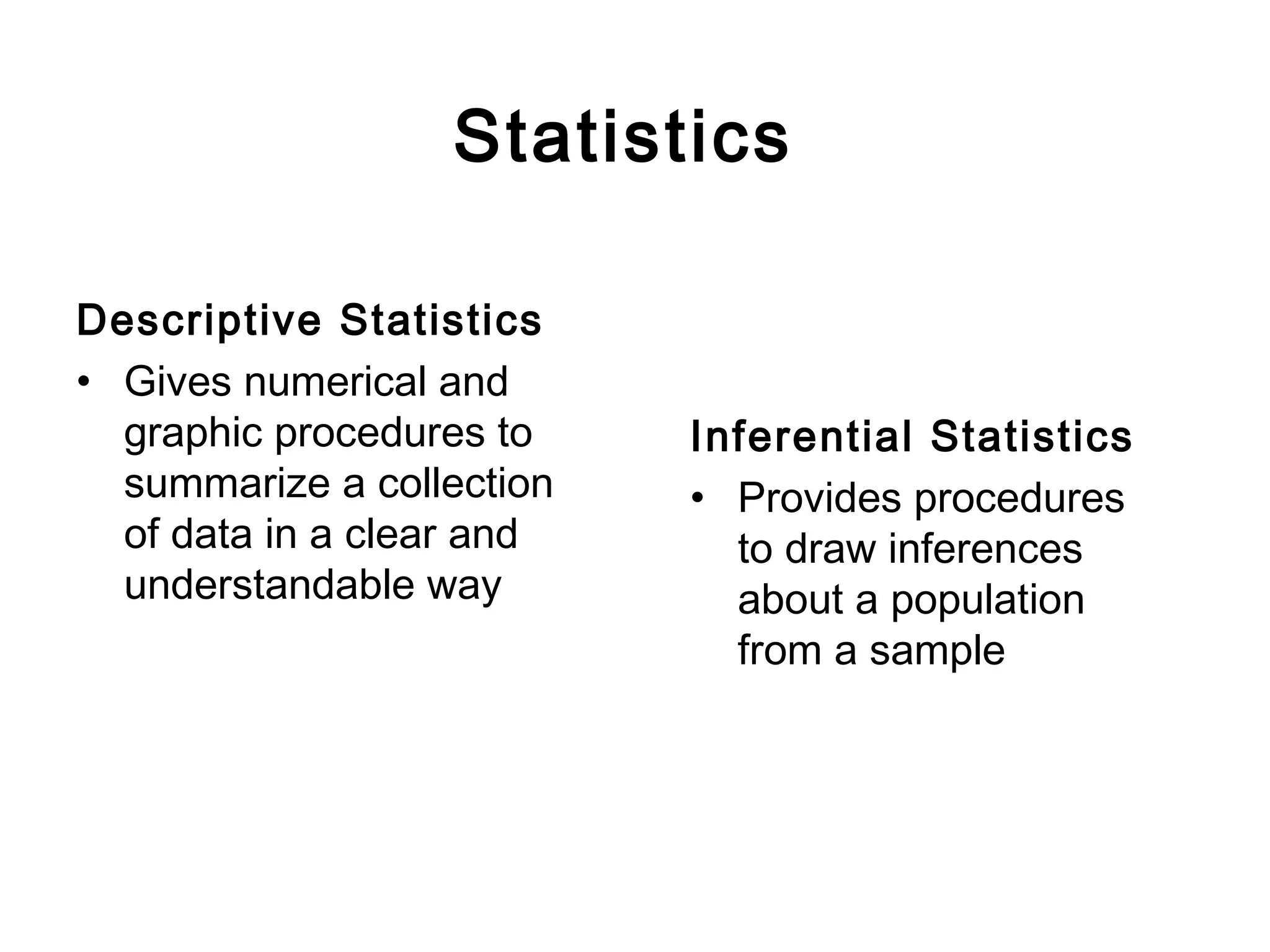
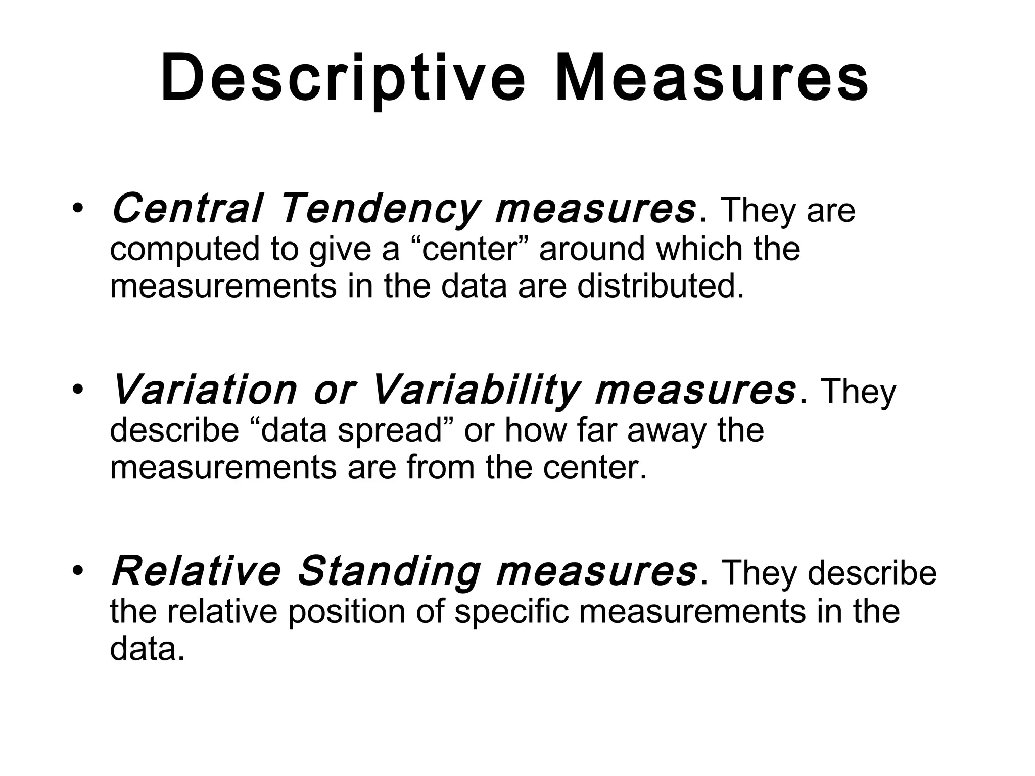
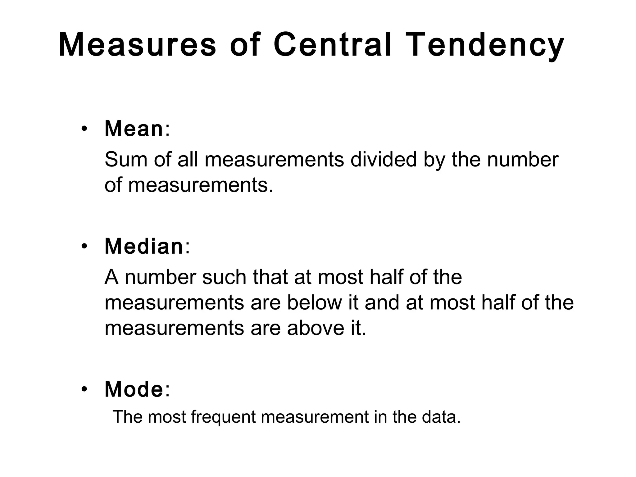
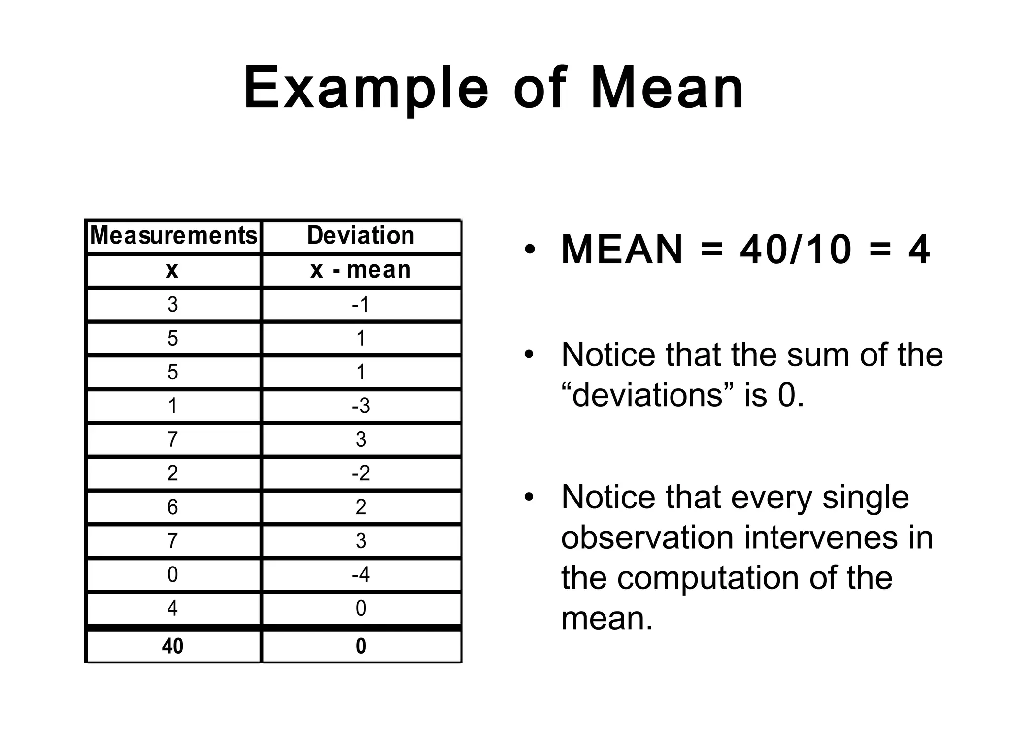
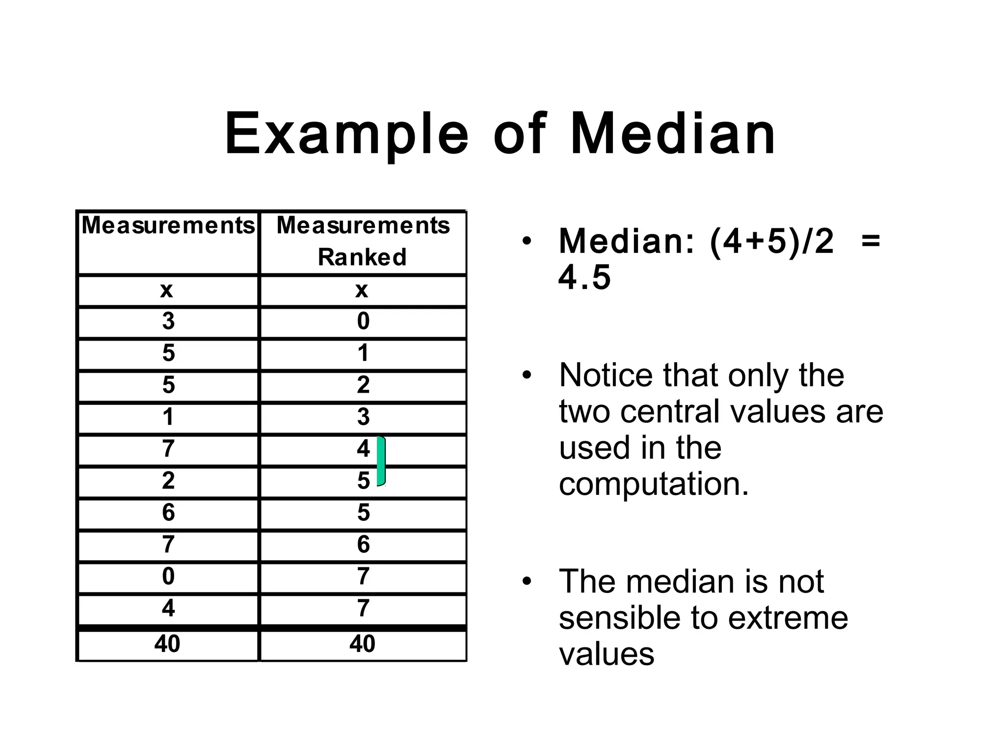
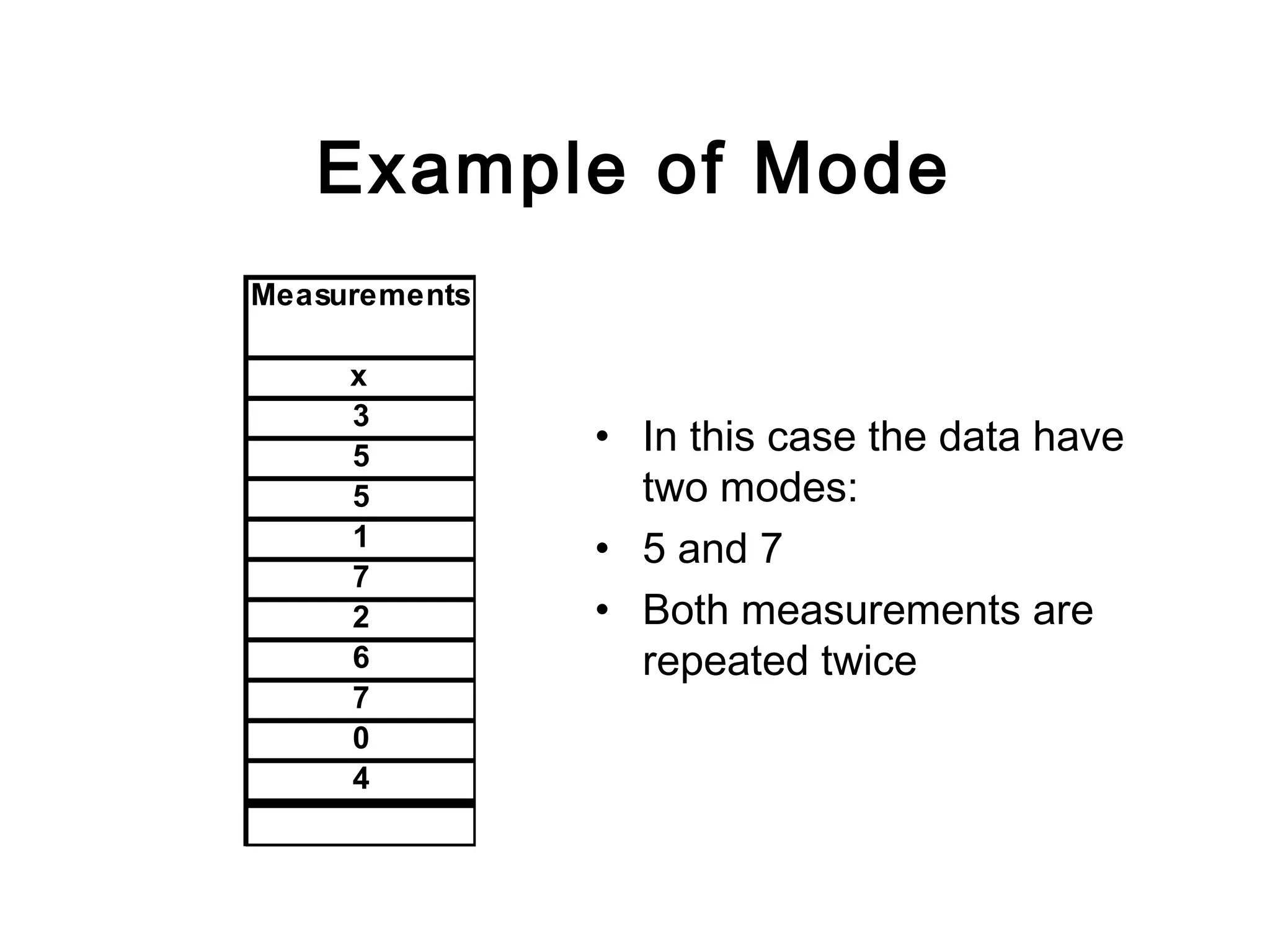
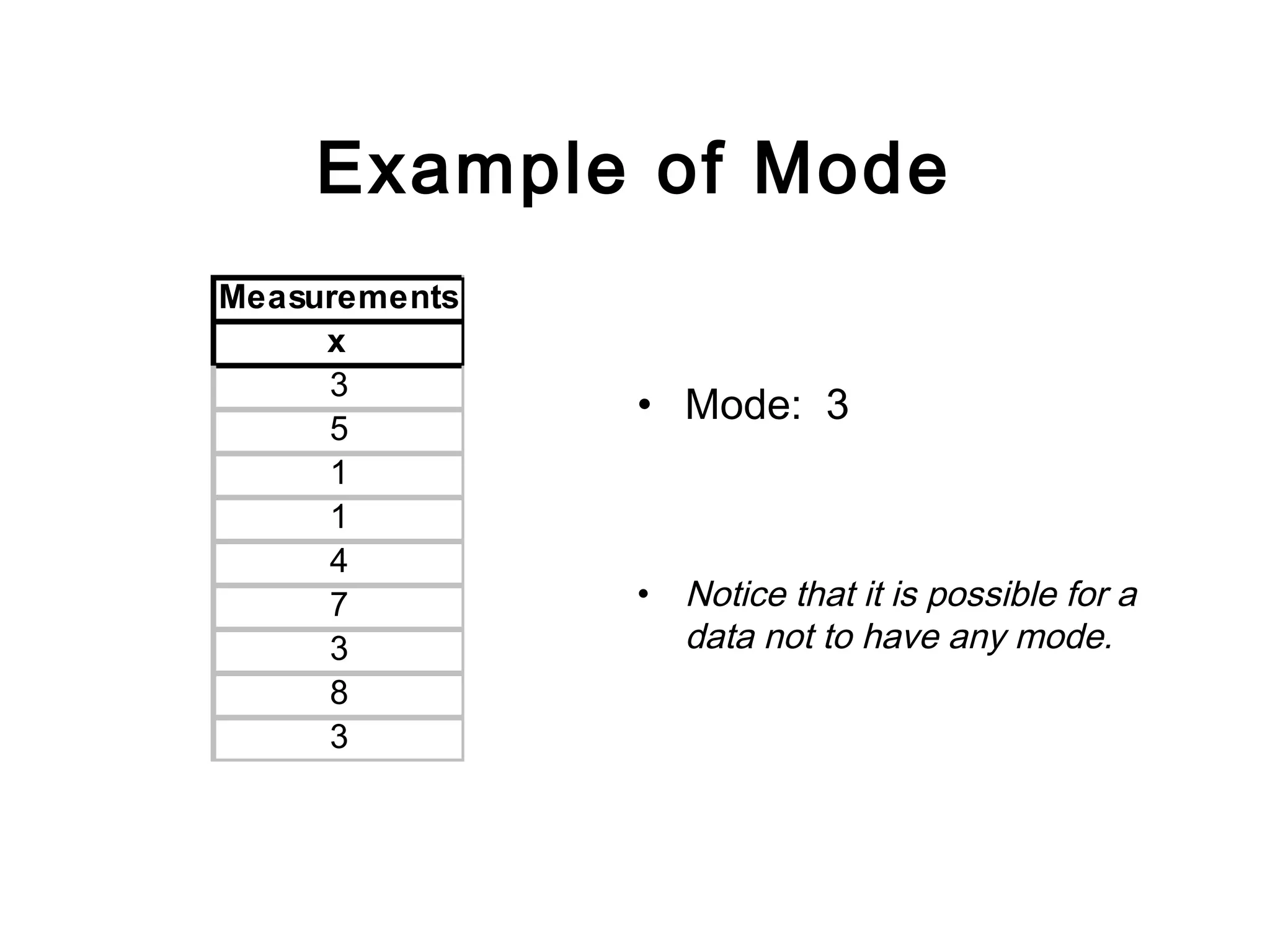
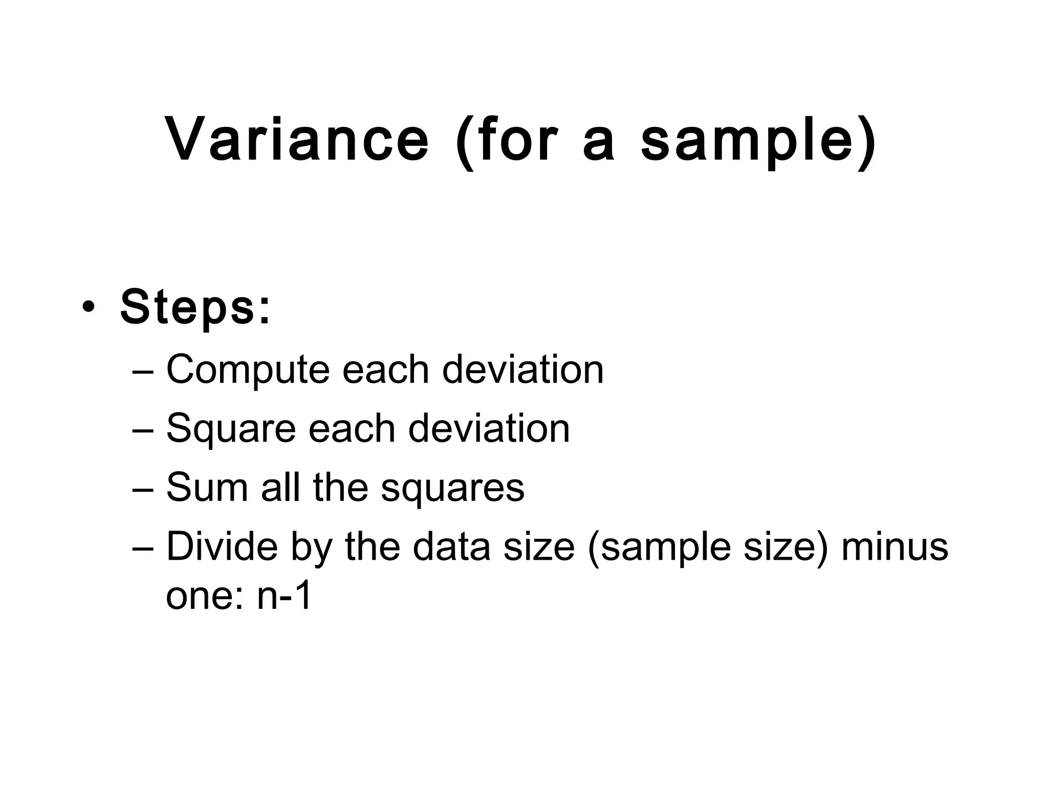
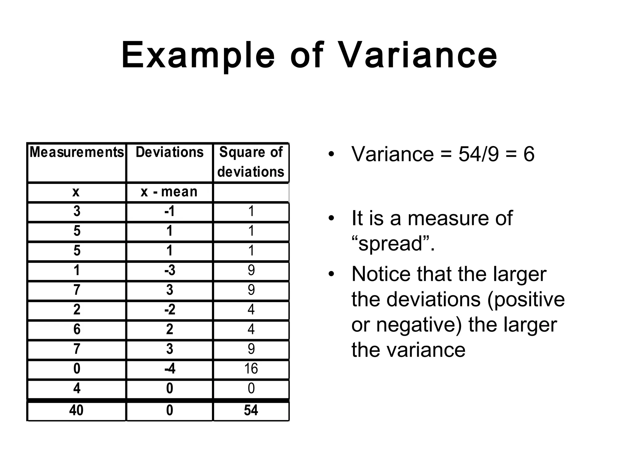
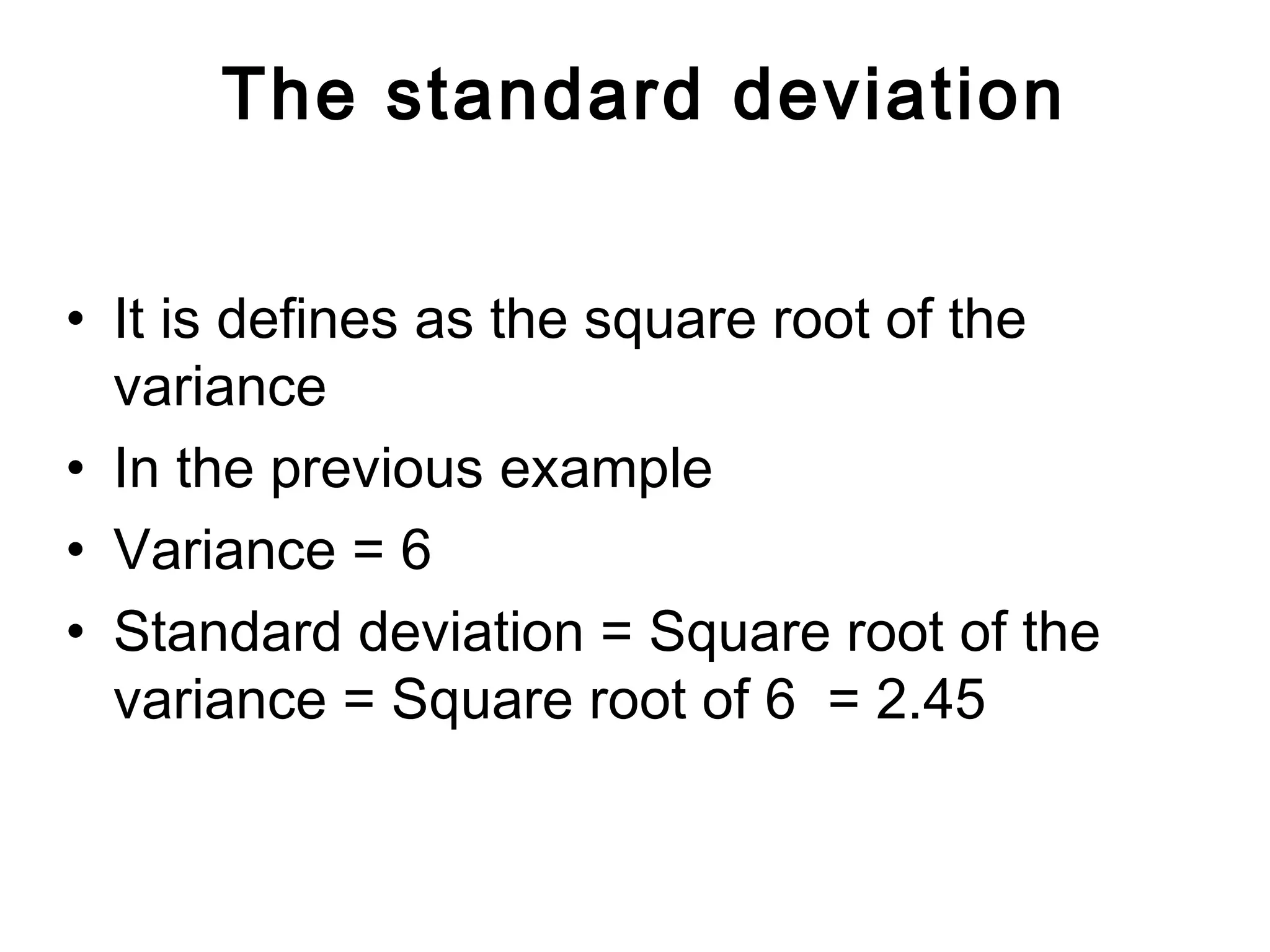
Descriptive statistics -review(2)

Descriptive statistics -review(2)

• 1.
  Descriptive Statistics for onevariable
• 2.
  Statistics has twomajor chapters: • Descriptive Statistics • Inferential statistics
• 3.
  Statistics Descriptive Statistics • Givesnumerical and graphic procedures to summarize a collection of data in a clear and understandable way Inferential Statistics • Provides procedures to draw inferences about a population from a sample
• 4.
  Descriptive Measures • CentralTendency measures. They are computed to give a “center” around which the measurements in the data are distributed. • Variation or Variability measures. They describe “data spread” or how far away the measurements are from the center. • Relative Standing measures. They describe the relative position of specific measurements in the data.
• 5.
  Measures of CentralTendency • Mean: Sum of all measurements divided by the number of measurements. • Median: A number such that at most half of the measurements are below it and at most half of the measurements are above it. • Mode: The most frequent measurement in the data.
• 6.
  Example of Mean MeasurementsDeviation x x - mean 3 -1 5 1 5 1 1 -3 7 3 2 -2 6 2 7 3 0 -4 4 0 40 0 • MEAN = 40/10 = 4 • Notice that the sum of the “deviations” is 0. • Notice that every single observation intervenes in the computation of the mean.
• 7.
  Example of Median •Median: (4+5)/2 = 4.5 • Notice that only the two central values are used in the computation. • The median is not sensible to extreme values Measurements Measurements Ranked x x 3 0 5 1 5 2 1 3 7 4 2 5 6 5 7 6 0 7 4 7 40 40
• 8.
  Example of Mode Measurements x 3 5 5 1 7 2 6 7 0 4 •In this case the data have two modes: • 5 and 7 • Both measurements are repeated twice
• 9.
  Example of Mode Measurements x 3 5 1 1 4 7 3 8 3 •Mode: 3 • Notice that it is possible for a data not to have any mode.
• 10.
  Variance (for asample) • Steps: – Compute each deviation – Square each deviation – Sum all the squares – Divide by the data size (sample size) minus one: n-1
• 11.
  Example of Variance MeasurementsDeviations Square of deviations x x - mean 3 -1 1 5 1 1 5 1 1 1 -3 9 7 3 9 2 -2 4 6 2 4 7 3 9 0 -4 16 4 0 0 40 0 54 • Variance = 54/9 = 6 • It is a measure of “spread”. • Notice that the larger the deviations (positive or negative) the larger the variance
• 12.
  The standard deviation •It is defines as the square root of the variance • In the previous example • Variance = 6 • Standard deviation = Square root of the variance = Square root of 6 = 2.45
• 13.
  Percentiles • The p-thepercentile is a number such that at most p% of the measurements are below it and at most 100 – p percent of the data are above it. • Example, if in a certain data the 85th percentile is 340 means that 15% of the measurements in the data are above 340. It also means that 85% of the measurements are below 340 • Notice that the median is the 50th percentile
• 14.
  For any data •At least 75% of the measurements differ from the mean less than twice the standard deviation. • At least 89% of the measurements differ from the mean less than three times the standard deviation. Note: This is a general property and it is called Tchebichev’s Rule: At least 1-1/k2 of the observation falls within k standard deviations from the mean. It is true for every dataset.
• 15.
  Example of Tchebichev’sRule Suppose that for a certain data is : • Mean = 20 • Standard deviation =3 Then: • A least 75% of the measurements are between 14 and 26 • At least 89% of the measurements are between 11 and 29
• 16.
  Further Notes • Whenthe Mean is greater than the Median the data distribution is skewed to the Right. • When the Median is greater than the Mean the data distribution is skewed to the Left. • When Mean and Median are very close to each other the data distribution is approximately symmetric.