Course Overview
• Thiscourse aims to provide students with a comprehensive
understanding of data analysis using Python.
• It covers various libraries, tools, and techniques necessary for
effective data manipulation, analysis, and visualization.
3.
Additional Resources
Books:
o"Python for Data Analysis" by Wes McKinney
o "Data Science from Scratch" by Joel Grus
Online Platforms:
o Kaggle, DataCamp, Coursera, edX
Practice Datasets:
o Titanic Dataset, Iris Dataset, Boston Housing Dataset
4.
Learning Outcomes
• Bythe end of this module, students will:
Understand the purpose and applications of data analysis.
Be familiar with the data analysis process.
Have a working Python environment with essential libraries
installed.
Be able to write and execute basic Python code in Jupyter
Notebook.
5.
Content
• What isData Analysis?
• Applications of Data Analysis
• Types of Data Analysis
• Data Analysis Process Steps
• Why Python for Data Analysis
• Setting Up the Environment
• Use Case Demo
What is DataAnalysis?
• Data analysis is the systematic process of :
– examining,
– cleaning,
– transforming, and
– modeling data to
• extract useful information,
• draw conclusions, and
• support decision-making.
• It often uses statistical analysis, machine learning, and other
computational tools to make sense of large and complex
datasets.
• It involves several key steps and techniques, including:
What is DataAnalysis?
• Key Components of Data Analysis
1. Data Collection:
Gathering data from various sources, such as surveys,
experiments, databases, or online platforms.
2. Data Cleaning:
Identifying and correcting errors or inconsistencies in the data to
ensure its quality and accuracy. This can include handling missing
values, removing duplicates, and correcting formatting issues.
3. Data Exploration:
Analyzing the data to discover patterns, trends, and relationships.
This often involves using descriptive statistics, visualizations, and
exploratory techniques.
4. Data Transformation:
Modifying the data into a suitable format for analysis. This may
involve aggregating, normalizing, or encoding data.
10.
What is DataAnalysis?
• Key Components of Data Analysis
5. Modeling:
Applying statistical or machine learning models to analyze the
data further, make predictions, or identify underlying structures.
6. Interpretation:
Drawing conclusions based on the analysis, understanding the
implications of the findings, and relating them to the initial questions or
business objectives.
7. Communication:
Presenting the results in a clear and effective manner, often
through visualizations, reports, or presentations, to stakeholders or
decision-makers.
11.
What is DataAnalysis?
• Importance of Data Analysis
• Informed Decision-Making:
• Helps organizations make data-driven decisions, reducing reliance on
intuition or guesswork.
• Identifying Trends:
• Enables the identification of trends and patterns that can inform business
strategies or scientific research.
• Problem Solving:
• Assists in diagnosing issues and determining effective solutions based on empirical
evidence.
• Forecasting:
• Provides insights into future trends by analyzing historical data, which can
aid in planning and resource allocation.
12.
Applications of DataAnalysis
• Business:
• Market analysis, customer segmentation, sales forecasting, and financial performance
evaluation.
• Healthcare:
• Patient data analysis, treatment effectiveness studies, and population health
management.
• Social Sciences:
• Survey data analysis, behavioral studies, and demographic research.
• Engineering:
• Quality control, product testing, and performance optimization(improvement}.
Types of DataAnalysis
• Descriptive Analytics:
• Summarizes historical data to understand what has happened. It uses measures
like averages, totals, and visualizations to provide insights.
• Diagnostic Analytics:
• Explores the reasons behind past outcomes. It looks into data to identify patterns
and correlations, helping to answer "why" something happened.
• Predictive Analytics:
• Uses statistical models and machine learning techniques to predict future outcomes
based on historical data. It answers questions like "what is likely to happen?"
• Prescriptive Analytics:
• Provides recommendations for actions based on the data analysis. It answers "what
should we do?" by suggesting optimal strategies or decisions.
Why Python forData Analysis
1. Ease of Learning and Use
• Readable Syntax: Python’s syntax is clear and intuitive, making it accessible for beginners and
allowing data analysts to focus on data manipulation rather than complex programming
constructs.
• Active Community: A large and active community means extensive resources, tutorials, and
forums are available for support.
2. Powerful Libraries
• Pandas: Offers data structures and functions specifically designed for data manipulation and
analysis. It simplifies tasks such as data cleaning, aggregation, and transformation.
• NumPy: Provides support for large, multi-dimensional arrays and matrices, along with
mathematical functions to operate on them.
• Matplotlib & Seaborn: These libraries are great for data visualization, allowing users to create
a wide range of static, animated, and interactive visualizations.
• SciPy: Useful for scientific and technical computing, it builds on NumPy and provides additional
functionality for optimization, integration, and statistics.
• Scikit-learn: A powerful library for machine learning that provides simple and efficient tools for
data mining and analysis.
28.
Why Python forData Analysis
3. Versatility
• General-Purpose Language: Python can be used for various programming tasks beyond data
analysis, such as web development, automation, and scripting, making it a versatile tool for
data professionals.
• Integration: Python can easily integrate with other languages and technologies, such as SQL
databases, APIs, and big data frameworks like Hadoop and Spark.
4. Support for Data Visualization
Visualization is a crucial aspect of data analysis, and Python provides numerous libraries (like
Matplotlib, Seaborn, and Plotly) that enable analysts to create informative and aesthetically pleasing
visual representations of data.
5. Jupyter Notebooks
Jupyter Notebooks offer an interactive environment for developing and presenting data analysis.
They allow users to combine code, visualizations, and narrative text, making it easier to share
insights and findings.
6. Scalability
Python can handle small to large datasets, and with libraries like Dask and PySpark, it can scale up
to big data processing tasks, making it suitable for various data analysis needs.
29.
Why Python forData Analysis
7. Machine Learning and AI Capabilities
Python is a leading language for machine learning and artificial intelligence, providing a seamless
transition from data analysis to building predictive models.
8. Cross-Platform Compatibility
Python is cross-platform, meaning that code written on one operating system can easily run on
others, providing flexibility for data analysts working in diverse environments.
30.
Setting Up theEnvironment
Installing Python and Jupyter Notebook:
o Download and install Python from python.org.
o Install Jupyter Notebook using pip: pip install notebook.
o Launch Jupyter Notebook: jupyter notebook.
Using Anaconda Distribution:
o Anaconda is a popular Python distribution for data analysis.
o Download and install Anaconda from anaconda.com.
o Use Anaconda Navigator to launch Jupyter Notebook and manage libraries.
o Create and manage virtual environments using Conda.
31.
Demo
• Analyzing aSample Dataset
• Let's assume we have a CSV file named sales_data.csv with the following
structure:
32.
Demo
• Step-by-Step Analysis
1.Import Libraries:
First, you'll need to import the necessary libraries.
• import pandas as pd
• import matplotlib.pyplot as plt
2. Load the Dataset:
Load the CSV file into a Pandas DataFrame.
# Load the data
df = pd.read_csv('sales_data.csv’)
3. Data Inspection:
Check the first few rows of the dataset to understand its structure.
print(df.head())
33.
Demo
• Step-by-Step Analysis
4.Basic Analysis:
Perform some basic analysis to get insights.
# Summary statistics
print(df.describe())
# Total sales and profit per product
total_sales = df.groupby('Product')['Sales'].sum()
total_profit = df.groupby('Product')['Profit'].sum()
print(total_sales)
print(total_profit)
34.
Demo
• Step-by-Step Analysis
5.Data Visualization:
Visualize the total sales per product using a bar chart.
total_sales.plot(kind='bar', title='Total Sales per Product')
plt.xlabel('Product')
plt.ylabel('Total Sales')
plt.show()
6. Running the Code
To run this code, you'll need to have Python and the necessary libraries
(Pandas and Matplotlib) installed. You can do this using pip:
pip install pandas matplotlib
35.
Hands-On Activities
1. InstallPython and Jupyter Notebook:
o Follow the installation steps and verify the setup.
2. Write a Simple Python Script:
o Create a script to perform basic operations (e.g., arithmetic calculations, string
manipulation).
3. Explore Jupyter Notebook:
o Create a new notebook, write code, and add markdown cells for documentation.
4. Install Key Libraries:
o Use pip or Conda to install NumPy, Pandas, Matplotlib, Seaborn, and Scikit-learn.
o Verify the installation by importing the libraries in a Python script.
36.
Data Analysis withPython
Dr.Ahmed Alnasheri Lecture 2
Practical introduction to Python
37.
Learning Outcomes
• Bythe end of this module, students will:
Understand the “common” aspects of Python programming
Understand the absolute basics of Python
38.
Interpretive vs compiled
languages
•Python is an interpretive language.
• This means that your code is not directly run by the hardware.
It is instead passed to a virtual machine, which is just another
programme that reads and interprets your code.
• This is in contrast to compiled languages, where your code is
translated into native machine instructions, which are then
directly executed by the hardware.
39.
Advantages of Python?
•Because Python is an interpretive language, it has a number
of advantages:
– Automatic memory management.
– Expressivity and syntax that is ‘English’.
– Ease of programming.
– Minimises development time.
– Python also has a focus on importing modules, a feature that makes it useful
for scientific computing.
40.
Disadvantages of Python?
•Interpreted languages are slower than compiled languages.
• The modules that you import are developed in a
decentralised manner; this can cause issues based upon
individual assumptions.
• Multi-threading is hard in Python
41.
Which language isthe best
• No one language is better
than all others.
• The ‘best’ language
depends on the task you
are using it for and your
personal preference.
42.
Versions of Python
•There are currently two versions of Python in use; Python 2
and Python 3.
• Python 3 is not backward compatible with Python 2.
• A lot of the imported modules were only available in Python
2 for quite some time, leading to a slow adoption of Python
3. However, this not really an issue anymore.
• Support for Python 2 was ended in 2020.
43.
The Anaconda IDE…
•The Anaconda distribution is the most
popular Python distribution out there.
• Most importable packages are pre-
installed.
• Offers a nice GUI in the form of Spyder.
• Before we go any further, let’s open
Spyder:
Variables
• Variables inpython can contain alphanumerical characters and some special
characters.
• By convention, it is common to have variable names that start with lower case letters
and have class names beginning with a capital letter; but you can do whatever you
want.
• Some keywords are reserved and cannot be used as variable names due to them
serving an in-built Python function; i.e. and, continue, break. Your IDE will let you know if
you try to use one of these.
• Python is dynamically typed; the type of the variable is derived from the value it is
assigned.
46.
Variable types
• Integer(int)
• Float (float)
• String (str)
• Boolean (bool)
• Complex (complex)
• […]
• User defined
(classes)
• A variable is assigned using the = operator; i.e:
In: Out:
• Create an integer, float, and string
variable.
• Print these to the screen.
• Play around using different variable
names, etc.
• The print() function is used to print
something to the screen.
47.
• You canalways check the type of a variable using the type() function.
In: Out:
• Check the type of one of your variables.
Variable types
48.
• Variables canbe cast to a different type.
In: Out:
Variable types
49.
Arithmetic operators
The arithmetic
operators:
•Addition: +
• Subtract: -
• Multiplication: *
• Division: /
• Power: **
• Write a couple of operations
using the arithmetic operators,
and print the results to the
screen.
In: Out:
50.
A quick noteon the increment
operator shorthand
• Python has a common idiom that is not necessary, but which is
used frequently and is therefore worth noting:
x += 1
Is the same as:
x = x + 1
• This also works for other operators:
x += y # adds y to the value of x
x *= y # multiplies x by the value y
x -= y # subtracts y from x
x /= y # divides x by y
51.
Boolean Operators
• Booleanoperators are useful when making
conditional statements, we will cover these
in-depth later.
– and
– or
– not
52.
Comparison operators
• Greaterthan: >
• Lesser than: <
• Greater than or equal to: >=
• Lesser than or equal to: <=
• Is equal to: ==
In:
Out:
• Write a couple of operations using
comparison operators; i.e.
53.
In: Out:
Working withstrings
• Create a string variable.
• Work out the length of the string.
Indexing
• Indexing inPython is 0-based, meaning that the first element in
a string, list, array, etc, has an index of 0. The second element
then has an index of 1, and so on.
In: Out:
• You can cycle backwards through a list, string, array, etc, by
placing a minus symbol in front of the index location.
In: Out:
56.
In: Out:
In: Out:
•Create a string that is 10 characters in length.
• Print the second character to the screen.
• Print the third to last character to the screen.
• Print all characters after the fourth character.
• Print characters 2-8.
Indexing
57.
Tuples
• Tuples arecontainers that are immutable; i.e.
their contents cannot be altered once created.
In: Out:
In: Out:
58.
Lists
• Lists areessentially containers of arbitrary
type.
• They are probably the container that you will
use most frequently.
• The elements of a list can be of different
types.
• The difference between tuples and lists is in
performance; it is much faster to ‘grab’ an
element stored in a tuple, but lists are much
more versatile.
• Note that lists are denoted by [] and not the ()
used by tuples.
In:
Out:
• Create a list and populate it with some elements.
59.
• Lists aremutable; i.e. their contents can be changed. This can be
done in a number of ways.
• With the use of an index to replace a current element with a new one.
In: Out:
Adding elements to a list
• Replace the second element in your list with the integer 2.
60.
• You canuse the insert() function in order to add an element to a
list at a specific indexed location, without overwriting any of the
original elements.
In: Out:
• Use insert() to put the integer 3 after the 2 that you just added to
your string.
Adding elements to a list
61.
• You canadd an element to the end of a list using the
append() function.
In: Out:
• Use append() to add the string “end” as the last element in your list.
Adding elements to a list
62.
Removing elements froma list
• You can remove an element from a list based
upon the element value.
• Remember: If there is more than one element
with this value, only the first occurrence will be
removed.
In: Out:
63.
• It isbetter practice to remove elements by their index using the
del function.
In: Out:
• Use del to remove the 3 that you added to the list earlier.
Removing elements from a list
64.
For loops
• Thefor loop is used to iterate over elements in a
sequence, and is often used when you have a piece of
code that you want to repeat a number of times.
• For loops essentially say:
“For all elements in a sequence, do something”
65.
An example
• Wehave a list of species:
• The command underneath the list then cycles through each entry in
the species list and prints the animal’s name to the screen. Note:
The i is quite arbitrary. You could just as easily replace it with
‘animal’, ‘t’, or anything else.
66.
Another example
• Wecan also use for loops for operations other than printing to a
screen. For example:
• Using the list you made a moment ago, use a for loop to print
each element of the list to the screen in turn.
67.
The range() function
•The range() function generates a list of numbers, which is generally used to
iterate over within for loops.
• The range() function has two sets of parameters to follow:
range(stop)
stop: Number of integers
(whole numbers) to generate,
starting from zero. i.e:
range([start], stop[, step])
start: Starting number of the sequence.
stop: Generate numbers up to, but not including this
number.
step: Difference between each number in the
sequence. i.e.:
Note:
• All parameters must be integers.
• Parameters can be positive or negative.
• The range() function (and Python in general) is 0-index based, meaning list indexes start at 0,
not 1. eg. The syntax to access the first element of a list is mylist[0]. Therefore the last
integer generated by range() is up to, but not including, stop.
68.
• Create anempty list.
• Use the range() and append() functions to add the
integers 1-20 to the empty list.
• Print the list to the screen, what do you have?
Output:
Creating list
69.
The break() function
•To terminate a loop, you can use the break()
function.
• The break() statement breaks out of the
innermost enclosing for or while loop.
70.
• The continue()statement is used to tell Python to
skip the rest of the statements in the current
loop block, and then to continue to the next
iteration of the loop.
The continue () function
71.
While loops
• Thewhile loop tells the computer to do something as long as a specific condition is
met.
• It essentially says:
“while this is true, do this.”
• When working with while loops, its important to remember the nature of various
operators.
• While loops use the break() and continue() functions in the same way as a for loop does.
• Create avariable and set it to zero.
• Write a while loop that states that, while the variable is
less than 250, add 1 to the variable and print the
variable to the screen.
• Replace the < with <=, what happens?
In: Out:
75.
For loop vs.while loop
• You will use for loops more often than while loops.
• The for loop is the natural choice for cycling through a list, characters in
a string, etc; basically, anything of determinate size.
• The while loop is the natural choice if you are cycling through
something, such as a sequence of numbers, an indeterminate number
of times until some condition is met.
76.
Nested loops
• Insome situations, you may want a loop within a loop;
this is known as a nested loop.
In:
Out:
• What will the code on the right
produce?
• Recreate this code and run it, what
do you get?
77.
Conditionals
• There arethree main conditional statements in
Python; if, else, elif.
• We have already used if when looking at while loops.
In: Out:
In: Out:
Functions
• A functionis a block of code which only
runs when it is called.
• They are really useful if you have
operations that need to be done
repeatedly; i.e. calculations.
• The function must be defined before it is
called. In other words, the block of code
that makes up the function must come
before the block of code that makes use of
the function.
In:
Out:
80.
In:
Out:
• Create afunction that takes two inputs, multiplies them, and then returns the
result. It should look some like:
def function_name(a, b):
do something
return something
• Create two different lists of integers.
• Using your function, write a nested for loop that cycles through each entries
in the first list and multiples it by each of the entries in the second list, and
prints the result to the screen.
Functions
Reading and writingto files in
Python: The file object
• File handling in Python can easily be done with the built-in
object file.
• The file object provides all of the basic functions necessary
in order to manipulate files.
• Open up notepad or notepad++. Write some text and save
the file to a location and with a name you’ll remember.
83.
The open() function
•Before you can work with a file, you first have to open it using Python’s
in-built open() function.
• The open() function takes two arguments; the name of the file that you
wish to use and the mode for which we would like to open the file
• By default, the open() function opens a file in ‘read mode’; this is what the ‘r’
above signifies.
• There are a number of different file opening modes. The most common
are: ‘r’ = read, ‘w’ =write, ‘r+’ =both reading and writing, ‘a’ =appending.
• Use the open() function to read the file in.
84.
The close() function
•Likewise, once you’re done working with a file, you can close it with the close() function.
• Using this function will free up any system resources that are being used up by having
the file open.
85.
Reading in afile and printing to
screen example
Using what you have now learned about for loops, it is
possible to open a file for reading and then print each
line in the file to the screen using a for loop.
• Use a for loop and the variable name that you assigned the open file
to in order to print each of the lines in your file to the screen.
In: Out:
86.
The read() function
•However, you don’t need to use any loops to access file contents. Python has
three in-built file reading commands:
1. <file>.read() = Returns the entire contents of the file as a single string:
2. <file>.readline() = Returns one line at a time:
3. <file>.readlines() = Returns a list of lines:
87.
The write() function
•Likewise, there are two similar in-built functions for
getting Python to write to a file:
1. <file>.write() = Writes a specified sequence of characters to a file:
2. <file>.writelines() = Writes a list of strings to a file:
• Important: Using the write() or writelines() function will overwrite anything contained
within a file, if a file of the same name already exists in the working directory.
88.
Practice – writingto a file in
Python
Part 1:
• Open the file you created in the last practice and ready it for being
written to.
• Write a string to that file. Note: this will overwrite the old contents.
• Remember to close the file once you are done.
Part 2:
• Create a list of strings.
• Use the open() function to create a new .txt file and write your list of
strings to this file.
• Remember to close the file once you are done.
89.
The append() function
•If you do not want to overwrite a file’s contents, you can use the append() function.
• To append to an existing file, simply put ‘a’ instead of ‘r’ or ‘w’ in the open() when
opening a file.
90.
Practice – appendingto a file
in Python
• Open the text file you created in part two of the writing to a file practice, and
ready it for appending.
• Define a string object.
• Appending this new string object to the file.
• Remember to close the file once you are done.
91.
A word onimport
• To use a package in your code, you must first make it
accessible.
• This is one of the features of Python that make it so
popular.
In:
• There are pre-built Python packages for pretty much
everything.
In:
92.
Plotting in Python
•Before creating an plots, it is worth spending
sometime familiarising ourselves with the matplotlib
module. It will save a lot of time later on.
93.
Some history….
• Matplotlibwas originally developed by a neurobiologist in order to emulate
aspects of the MATLAB software.
• The pythonic concept of importing is not utilised by MATLAB, and this is
why something called Pylab exists.
• Pylab is a module within the Matplotlib library that was built to mimic the
MATLAB style. It only exists in order to bring aspects of NumPy and Matplotlib
into the namespace, thus making for an easier transition for ex-MATLAB
users, because they only had to do one import in order to access the
necessary functions:
• However, using the above command is now considered bad
practice, and Matplotlib actually advises against using it due to the
way in which it creates many opportunities for conflicted name
bugs.
94.
Getting started
• WithoutPylab, we can normally get away with just one
canonical import; the top line from the example below.
• We are also going to import NumPy, which we are going to
use to generate random data for our examples.
95.
Different graph types
•A simple line graph can be plotted with plot().
• A histogram can be created with hist().
• A bar chart can be created with bar().
• A pie chart can be created with pie().
• A scatter plot can be created with scatter().
• The table() function adds a text table to an axes.
• Plus many more….
96.
Our first plot
•You may be wondering why the x-axis ranges
from 0-3 and the y-axis from 1-4.
• If you provide a single list or array to the plot()
command, Matplotlib assumes it is a
sequence of y values, and automatically
generates the x values for you.
• Since python ranges start with 0, the default
x vector has the same length as y but starts
with 0.
• Hence the x data are [0,1,2,3].
97.
The plot() function
•The plot() argument is quite
versatile, and will take any
arbitrary collection of numbers.
For example, if we add an extra
entry to the x axis, and replace the
last entry in the Y axis and add
another entry:
98.
The plot() function
•The plot() function has an optional third argument that
specifies the appearance of the data points.
• The default is b-, which is the blue solid line seen in the
last two examples. The full list of styles can be found in
the documentation for the plot() on the Matplotlib page
99.
The plot() function
•You can quite easily alter the properties of the line with
the plot() function.
100.
Altering tick labels
•The plt.xticks() and plt.yticks()
allows you to manually
alter the ticks on the x-
axis and y-axis
respectively.
• Note that the tick values
have to be contained
within a list object.
101.
Practice - Basicline graph
Let’s write a Python program to draw a line graph with suitable
labels for the x-axis and y-axis. Include a title.
102.
The setp() function
•The setp() allows you to set multiple properties for a list of lines, if you want
all the lines to be matching.
• You can use the setp() function along with either the line or lines function in order
to get a list of settable line properties.
103.
The axis() function
•The axis() function allows us to specify the range of the axis.
• It requires a list that contains the following:
[The min x-axis value, the max x-axis value, the min y-axis, the max y-axis value]
104.
Matplotlib and NumPyarrays
• Normally when working with numerical data, you’ll be
using NumPy arrays.
• This is still straight forward to do in Matplotlib; in fact all
sequences are converted into NumPy arrays internally
anyway.
105.
Working with text
•There are a number of different ways in which to add
text to your graph:
- title() = Adds a title to your graph,
takes a string as an argument
- xlabel() = Add a title to the x-axis, also
takes a string as an argument
- ylabel() = Same as xlabel()
- text() = Can be used to add text to an
arbitrary location on your graph.
. Requires the following arguments:
text(x-axis location, y-axis location, the string
. of text to be added)
• Matplotlib uses TeX equation expressions. So, as an
example, if you wanted to put in one of the text
blocks, you would write plt.title(r'$sigma_i=15$').
106.
Annotating data points
•The annotate() function allows you to easily annotate
data points or specific area on a graph.
107.
Legends
• The locationof a legend is
specified by the loc command.
There are a number of in-built
locations that can be altered by
replacing the number. The
Matplotlib website has a list of all
locations in the documentation
page for location().
• You can then use the bbox_to_anchor()
function to manually place the
legend, or when used with loc, to
make slight alterations to the
placement.
108.
Saving a figureas a file
• The plt.savefig() allows you to
save your plot as a file.
• It takes a string as an
argument, which will be the
name of the file. You must
remember to state which
file type you want the figure
saved as; i.e. png or jpeg.
• Make sure you put the
plt.savefig() before the plt.show()
function. Otherwise, the file
will be a blank file.
109.
Scatter plot exercise
Let’swrite a Python program to plot quantities which
have an x and y position; a scatter graph.
110.
Debugging
• Debugging isin fundamental aspect of coding, and you will probably
spend more time debugging than actually writing code.
• EVERYONE has to debug, it is nothing to be ashamed of.
• In fact, you should be particularly concerned if you do write a
programme that does not display any obvious errors, as it likely
means that you are just unaware of them.
• There are a number of debugging programmes available to coders.
However, debugging the most common issues that you’ll encounter
when developing programmes can be done by following a few key
principles.
• However, always remember that sometimes
fixing a bug can create new bugs.
111.
Print everything
• Whendebugging, the most important function at your
disposal is the print command. Every coder uses this as a
debugging tool, regardless of their amount of experience.
• You should have some sense as to what every line of
code you have written does. If not, print those lines out.
You will then be able to see how the values of variables
are changing as the programme runs through.
• Even if you think you know what each line does, it is still
recommended that you print out certain lines as often this
can aid you in realising errors that you may have
overlooked.
112.
Print examples
I wantthe value of variable to be 10
upon completion of the for loop. Did
the for loop work correctly?
Yes, it did.
Did this chunk of code run?
No.
113.
Run your codewhen you make
changes
• Do not sit down and code for a hour or so without running
the code you are writing. Chances are, you will never get
to the bottom of all of the errors that your programme
reports when it runs.
• Instead, you should run your script every few minutes. It is
not possible to run your code too many times.
• Remember, the more code you write or edit between test
runs, the more places you are going to have to go back an
investigate when your code hits an error.
114.
Read your errormessages
• Do not be disheartened when you get an error message.
More often than not, you’ll realise what the error is as soon
as you read the message; i.e. the for loop doesn’t work on
a list because the list is empty.
• This is particularly the case with Python, which provides
you with error messages in ‘clear English’ compared to the
cryptic messages given by offered by other languages.
• At the very least, the error message will let you know which
lines is experiencing the error. However, this may not be
the line causing the error. Still, this offers a good starting
point for your bug search.
115.
Google the errormessage
• This can sometimes be a bit of a hit-or-miss, depending on the nature of the error.
• If your error is fairly specific, then there will nearly always be a webpage where
someone has already asked for help with an error that is either identical or very
similar to the one you are experiencing; stackoverflow.com is the most common
page you’ll come across in this scenario.
• Do make sure that you read the description
of the problem carefully to ensure that the
problem is the same as the one you are
dealing with. Then read the first two or three
replies to see if page contains a workable
solution.
• If you cannot work out the cause of an error
message, google the error code and
description.
116.
Comment out code
•You can often comment out bits of code that are
not related to the chunk of code that contains the
error.
• This will obviously make the code run faster and
might make it easier to isolate the error.
117.
Binary searches
• Thismethod draws upon a lot of the methods we
have already covered.
• Here, you want to break the code into chunks;
normally two chunks, hence this method’s name.
• You then isolate which chunk of code the error is
in.
• After which, you take the chunk of code in
question, and divide that up, and work out which
of these new chunks contains the error.
• So on until you’ve isolate the cause of the error.
118.
Walk away
• Ifyou have been trying to fix an error for a
prolonged period of time, 30 minutes or
so, get up and walk away from the screen
and do something else for a while.
• Often the answer to your issue will present
itself upon your return to the computer, as
if by magic.
119.
Phrase your problemas a
question
• Many software developers have
been trained to phrase their
problem as a question.
• The idea here is that phrasing
your issue in this manner often
helps you to realise the cause of
the problem.
• This often works!
120.
Ask someone
• Ifall else fails, do not hesitate to ask a colleague
or friend who is a coder and maybe familiar with
the language for help.
• They may not even need to be a specialist,
sometimes a fresh pair of eyes belonging to
someone who is not invested in the project is
more efficient at helping you work out your issue
than spending hours trying to solve the issue on
your own or getting lost the internet trying to find
a solution.
121.
Useful resources
• Thereare two great online resources for
learning this language through practical
examples. These are the Code Academy (
https://www.codecademy.com/catalog/subje
ct/web-development
) and Data Camp (
https://www.datacamp.com/?utm_source=a
dwords_ppc&utm_campaignid=805200711
&utm_adgroupid=39268379982&utm_devic
e=c&utm_keyword=data%20camp&utm_m
atchtype=e&utm_network=g&utm_adpostio
122.
Data Analysis withPython
Dr.Ahmed Alnasheri Lecture 3
Data Manipulation with
NumPy and Pandas
123.
Learning Outcomes
• Bythe end of this module, students will:
Understand the purpose and advantages of NumPy for
numerical computations.
Create and manipulate NumPy arrays.
Apply mathematical and statistical operations on arrays.
Understand the purpose and advantages of Pandas for data
manipulation and analysis.
Work with Pandas Data Structures.
Perform Data Cleaning and Preprocessing.
Perform Data Selection and Filtering.
Perform Data Transformation
124.
NumPy
• Stands forNumerical Python
• Is the fundamental package required for high performance
computing and data analysis
• NumPy is so important for numerical computations in Python is
because it is designed for efficiency on large arrays of data.
• It provides
– ndarray for creating multiple dimensional arrays
– Internally stores data in a contiguous block of memory, independent of
other built-in Python objects, use much less memory than built-in
Python sequences.
– Standard math functions for fast operations on entire arrays of data
without having to write loops
– NumPy Arrays are important because they enable you to express
batch operations on data without writing any for loops. We call this
vectorization.
125.
NumPy ndarray vslist
• One of the key features of NumPy is its N-dimensional
array object, or ndarray, which is a fast, flexible container
for large datasets in Python.
• Whenever you see “array,” “NumPy array,” or “ndarray” in
the text, with few exceptions they all refer to the same
thing: the ndarray object.
• NumPy-based algorithms are generally 10 to 100 times
faster (or more) than their pure Python counterparts and
use significantly less memory.
import numpy as np
my_arr = np.arange(1000000)
my_list = list(range(1000000))
126.
ndarray
• ndarray isused for storage of homogeneous data
– i.e., all elements the same type
• Every array must have a shape and a dtype
• Supports convenient slicing, indexing and efficient
vectorized computation
import numpy as np
data1 = [6, 7.5, 8, 0, 1]
arr1 = np.array(data1)
print(arr1)
print(arr1.dtype)
print(arr1.shape)
print(arr1.ndim)
[6. 7.5 8. 0. 1. ]
float64
(5,)
1
127.
Creating ndarrays
Using listof lists
import numpy as np
data2 = [[1, 2, 3, 4], [5, 6, 7, 8]] #list of lists
arr2 = np.array(data2)
print(arr2.ndim) #2
print(arr2.shape) # (2,4)
Arithmatic with NumPyArrays
• Arithmetic operations with scalars propagate the scalar argument to
each element in the array:
• Comparisons between arrays of the same size yield boolean arrays:
arr = np.array([[1., 2., 3.], [4., 5., 6.]])
print(arr)
[[1. 2. 3.]
[4. 5. 6.]]
print(arr **2)
[[ 1. 4. 9.]
[16. 25. 36.]]
arr2 = np.array([[0., 4., 1.], [7., 2., 12.]])
print(arr2)
[[ 0. 4. 1.]
[ 7. 2. 12.]]
print(arr2 > arr)
[[False True False]
[ True False True]]
131.
Indexing and Slicing
•One-dimensional arrays are simple; on the
surface they act similarly to Python lists:
arr = np.arange(10)
print(arr) # [0 1 2 3 4 5 6 7 8 9]
print(arr[5]) #5
print(arr[5:8]) #[5 6 7]
arr[5:8] = 12
print(arr) #[ 0 1 2 3 4 12 12 12 8 9]
132.
Indexing and Slicing
•As you can see, if you assign a scalar value to a slice, as in arr[5:8] =
12, the value is propagated (or broadcasted) to the entire selection.
• An important first distinction from Python’s built-in lists is that array
slices are views on the original array.
– This means that the data is not copied, and any modifications to the view
will be reflected in the source array.
arr = np.arange(10)
print(arr) # [0 1 2 3 4 5 6 7 8 9]
arr_slice = arr[5:8]
print(arr_slice) # [5 6 7]
arr_slice[1] = 12345
print(arr) # [ 0 1 2 3 4 5 12345 7 8 9]
arr_slice[:] = 64
print(arr) # [ 0 1 2 3 4 64 64 64 8 9]
133.
Indexing
• In atwo-dimensional array, the elements at each index are
no longer scalars but rather one-dimensional arrays:
• Thus, individual elements can be accessed recursively.
But that is a bit too much work, so you can pass a comma-
separated list of indices to select individual elements.
• So these are equivalent:
arr2d = np.array([[1, 2, 3], [4, 5, 6], [7, 8, 9]])
print(arr2d[2]) # [7 8 9]
print(arr2d[0][2]) # 3
print(arr2d[0, 2]) #3
134.
Activity
• Consider thetwo-dimensional array, arr2d.
• Write a code to slice this array to display the last
column,
[[3] [6] [9]]
• Write a code to slice this array to display the last
2 elements of middle array,
[5 6]
arr2d = np.array([[1, 2, 3], [4, 5, 6], [7, 8, 9]])
135.
Why pandas?
• Oneof the most popular library that data scientists use
• Labeled axes to avoid misalignment of data
– When merge two tables, some rows may be different
• Missing values or special values may need to be removed or replaced
height Weight Weight2 age Gender
Amy 160 125 126 32 2
Bob 170 167 155 -
1 1
Chris 168 143 150 28 1
David 190 182 NA 42 1
Ella 175 133 138 23 2
Frank 172 150 148 45 1
salary Credit score
Alice 50000 700
Bob NA 670
Chris 60000 NA
David -
99999 750
Ella 70000 685
Tom 45000 660
136.
Pandas Overview
• Createdby Wes McKinney in 2008, now
maintained by many others.
– Author of one of the textbooks: Python for Data
Analysis
• Powerful and productive Python data analysis
and Management Library
• Panel Data System
– The name is derived from the term "panel data",
an econometrics term for data sets that include
both time-series and cross-sectional data
• Its an open source product.
137.
Pandas Overview
• PythonLibrary to provide data analysis features similar
to: R, MATLAB, SAS
• Rich data structures and functions to make working with
data structure fast, easy and expressive.
• It is built on top of NumPy
• Key components provided by Pandas:
– Series
– DataFrame
from pandas import Series, DataFrame
import pandas as pd
From now on:
138.
Series
• One dimensionalarray-like object
• It contains array of data (of any NumPy data type) with
associated indexes. (Indexes can be strings or integers
or other data types.)
• By default , the series will get indexing from 0 to N where
N = size -1
from pandas import Series, DataFrame
import pandas as pd
obj = Series([4, 7, -5, 3])
print(obj)
print(obj.index)
print(obj.values)
#Output
0 4
1 7
2 -5
3 3
dtype: int64
RangeIndex(start=0, stop=4, step=1)
[ 4 7 -5 3]
139.
Series – referencingelements
obj2 = Series([4, 7, -5, 3], index=['d', 'b', 'a', 'c'])
print(obj2)
#Output
d 4
b 7
a -5
c 3
dtype: int64
print(obj2.index)
#Output
Index(['d', 'b', 'a', 'c'], dtype='object')
print(obj2.values)
#Output
[ 4 7 -5 3]
print(obj2['a'])
#Output
-5
obj2['d']= 10
print(obj2[['d', 'c', 'a']])
#Output
d 10
c 3
a -5
dtype: int64
print(obj2[:2])
#Output
d 10
b 7
dtype: int64
print(obj2.a)
#Output
-5
140.
Series – array/dictoperations
numpy array operations can also be applied,
which will preserve the index-value link
obj4 = obj3[obj3>0]
print(obj4)
#output
d 10
b 7
c 3
dtype: int64
print(obj3**2)
#output
d 100
b 49
a 25
c 9
dtype: int64
print(‘b’ in obj3)
#output
true
Can be thought of as a dict.
Can be constructed from a dict directly.
obj3 = Series({'d': 4, 'b': 7, 'a': -5, 'c':3 })
print(obj3)
#output
d 4
b 7
a -5
c 3
dtype: int64
Series name andindex name
sdata = {'Texas': 10, 'Ohio': 20, 'Oregon': 15, 'Utah': 18}
states = ['Texas', 'Ohio', 'Oregon', 'Iowa']
obj4 = Series(sdata, index=states)
obj4.name = 'population'
obj4.index.name = 'state'
print(obj4)
#output
state
Texas 10.0
Ohio 20.0
Oregon 15.0
Iowa NaN
Name: population, dtype: float64
144.
Series name andindex name
• Index of a series can be changed to a different index.
obj4.index = ['Florida', 'New York', 'Kentucky', 'Georgia']
Florida 10.0
New York 20.0
Kentucky 15.0
Georgia NaN
Name: population, dtype: float64
• Index object itself is immutable.
obj4.index[2]='California'
TypeError: Index does not support mutable operations
print(obj4.index)
Index(['Florida', 'New York', 'Kentucky', 'Georgia'], dtype='object')
145.
Indexing, selection andfiltering
• Series can be sliced/accessed with label-based
indexes, or using position-based indexes
S = Series(range(4), index=['zero', 'one', 'two', 'three'])
print(S['two'])
2
print(S[['zero', 'two']])
zero 0
two 2
dtype: int64
print(S[2])
2
print(S[[0,2]])
zero 0
two 2
dtype: int64
list operator for items >1
146.
Indexing, selection andfiltering
• Series can be sliced/accessed with label-based
indexes, or using position-based indexes
S = Series(range(4), index=['zero', 'one', 'two', 'three'])
print(S[:2])
zero 0
one 1
dtype: int32
print(S['zero': 'two'])
zero 0
one 1
two 2
dtype: int32
Inclusive
print(S[S > 1])
two 2
three 3
dtype: int32
print(S[-2:])
two 2
three 3
dtype: int32
147.
Activity
• Create arandom list of 10 integers in the range from 1
to 100
• Generate a Series using above list with index values of
1-10
– Name your Series “Random Numbers”
– Name your index “idx”
• Now generate the Squares of all the values in the
Series
– display last 4 items of this Series
– Also display all the numbers >500 as a list (without the
index)
148.
DataFrame
• A DataFrameis a tabular data structure comprised of rows and
columns, akin to a spreadsheet or database table.
• It can be treated as an ordered collection of columns
– Each column can be a different data type
– Have both row and column indices
data = {'state': ['Ohio', 'Ohio', 'Ohio', 'Nevada', 'Nevada'],
'year': [2000, 2001, 2002, 2001, 2002],
'pop': [1.5, 1.7, 3.6, 2.4, 2.9]}
frame = DataFrame(data)
print(frame)
#output
state year pop
0 Ohio 2000 1.5
1 Ohio 2001 1.7
2 Ohio 2002 3.6
3 Nevada 2001 2.4
4 Nevada 2002 2.9
149.
DataFrame – specifying
columnsand indices
• Order of columns/rows can be specified.
• Columns not in data will have NaN.
frame2 = DataFrame(data, columns=['year', 'state', 'pop', 'debt'], index=['A', 'B', 'C', 'D', 'E'])
Print(frame2)
year state pop debt
A 2000 Ohio 1.5 NaN
B 2001 Ohio 1.7 NaN
C 2002 Ohio 3.6 NaN
D 2001 Nevada 2.4 NaN
E 2002 Nevada 2.9 NaN
Same order
Initialized with NaN
150.
DataFrame – fromnested dict of
dicts
• Outer dict keys as columns and inner dict keys as row indices
pop = {'Nevada': {2001: 2.9, 2002: 2.9}, 'Ohio': {2002: 3.6, 2001: 1.7, 2000: 1.5}}
frame3 = DataFrame(pop)
print(frame3)
#output
Nevada Ohio
2000 NaN 1.5
2001 2.9 1.7
2002 2.9 3.6
print(frame3.T)
2000 2001 2002
Nevada NaN 2.9 2.9
Ohio 1.5 1.7 3.6
Transpose
Union of inner keys (in sorted order)
DataFrame – retrievinga
column
• A column in a DataFrame can be retrieved as a Series
by dict-like notation or as attribute
data = {'state': ['Ohio', 'Ohio', 'Ohio', 'Nevada', 'Nevada'],
'year': [2000, 2001, 2002, 2001, 2002],
'pop': [1.5, 1.7, 3.6, 2.4, 2.9]}
frame = DataFrame(data)
print(frame['state'])
0 Ohio
1 Ohio
2 Ohio
3 Nevada
4 Nevada
Name: state, dtype: object
print(frame.state)
0 Ohio
1 Ohio
2 Ohio
3 Nevada
4 Nevada
Name: state, dtype: object
153.
Activity
• Download thefollowing csv file and load it to
your python module or use the url directly in
pd.read_csv(url) which will read it to a
DataFrame
–
https://www.cs.odu.edu/~sampath/courses/f19/cs62
0/files/data/values.csv
• Calculate the average and standard deviation
(std) of the column factor_1 and display the
result.
– Pandas mean() and std()
154.
DataFrame – gettingrows
• loc for using indexes and iloc for using positions
– loc gets rows (or columns) with particular labels from the index.
– iloc gets rows (or columns) at particular positions in the index (so it only takes integers).
data = {'state': ['Ohio', 'Ohio', 'Ohio', 'Nevada', 'Nevada'],
'year': [2000, 2001, 2002, 2001, 2002],
'pop': [1.5, 1.7, 3.6, 2.4, 2.9]}
frame2 = DataFrame(data, columns=['year', 'state', 'pop', 'debt'], index=['A', 'B', 'C', 'D', 'E'])
print(frame2)
year state pop debt
A 2000 Ohio 1.5 NaN
B 2001 Ohio 1.7 NaN
C 2002 Ohio 3.6 NaN
D 2001 Nevada 2.4 NaN
E 2002 Nevada 2.9 NaN
print(frame2.loc['A'])
year 2000
state Ohio
pop 1.5
debt NaN
Name: A, dtype: object
print(frame2.loc[['A', 'B']])
year state pop debt
A 2000 Ohio 1.5 NaN
B 2001 Ohio 1.7 NaN
print(frame2.loc['A':'E',
['state','pop']])
state pop
A Ohio 1.5
B Ohio 1.7
C Ohio 3.6
D Nevada 2.4
E Nevada 2.9
print(frame2.iloc[1:3])
year state pop debt
B 2001 Ohio 1.7 NaN
C 2002 Ohio 3.6 NaN
print(frame2.iloc[:,1:3])
state pop
A Ohio 1.5
B Ohio 1.7
C Ohio 3.6
D Nevada 2.4
E Nevada 2.9
155.
DataFrame – modifying
columns
frame2['debt']= 0
print(frame2)
year state pop debt
A 2000 Ohio 1.5 0
B 2001 Ohio 1.7 0
C 2002 Ohio 3.6 0
D 2001 Nevada 2.4 0
E 2002 Nevada 2.9 0
frame2['debt'] = range(5)
print(frame2)
year state pop debt
A 2000 Ohio 1.5 0
B 2001 Ohio 1.7 1
C 2002 Ohio 3.6 2
D 2001 Nevada 2.4 3
E 2002 Nevada 2.9 4
val = Series([10, 10, 10], index = ['A', 'C', 'D'])
frame2['debt'] = val
print(frame2)
year state pop debt
A 2000 Ohio 1.5 10.0
B 2001 Ohio 1.7 NaN
C 2002 Ohio 3.6 10.0
D 2001 Nevada 2.4 10.0
E 2002 Nevada 2.9 NaN
Rows or individual elements can be
modified similarly. Using loc or iloc.
Activity
• Create anumpy array of the shape (3,5): 3
rows and 5 columns with random values from
1 to 100
– Use np.random.randint(low,high, (shape))
• Use the numpy array to generate a Data
Frame with index = a,b,c and columns 1,2,3,4,
5
• Transpose (using .T) the DataFrame and
change the values less than 40 to 0 in the
Data Frame.
Reindexing
• Alter theorder of rows/columns of a DataFrame or order of a series
according to new index
frame2 = frame.reindex(columns=['c2', 'c3', 'c1'])
print(frame2)
c2 c3 c1
r1 1 2 0
r2 4 5 3
r3 7 8 6
frame2 = frame.reindex(['r1', 'r3', 'r2', 'r4'])
c1 c2 c3
r1 0.0 1.0 2.0
r3 6.0 7.0 8.0
r2 3.0 4.0 5.0
r4 NaN NaN NaN
This returns a new object
163.
Function application and
mapping
•DataFrame.applymap(f) applies f to every entry
• DataFrame.apply(f) applies f to every column (default) or row
def max_minus_min(x):
return max(x)-min(x)
print(frame.apply(max_minus_min))
c1 6
c2 6
c3 6
dtype: int64
print(frame.apply(max_minus_min,axis=1))
r1 2
r2 2
r3 2
dtype: int64
print(frame)
c1 c2 c3
r1 0 1 2
r2 3 4 5
r3 6 7 8
def square(x):
return x**2
print(frame.applymap(square))
c1 c2 c3
r1 0 1 4
r2 9 16 25
r3 36 49 64
164.
Function application and
mapping
defmax_min(x):
return Series([max(x), min(x)], index=['max', 'min'])
print(frame.apply(max_min))
c1 c2 c3
max 6 7 8
min 0 1 2
165.
Other DataFrame functions
•sort_index()
frame.index=['A', 'C', 'B'];
frame.columns=['b','a','c'];
print(frame)
b a c
A 0 1 2
C 3 4 5
B 6 7 8
print(frame.sort_index())
b a c
A 0 1 2
B 6 7 8
C 3 4 5
print(frame.sort_index(axis=1))
a b c
A 1 0 2
C 4 3 5
B 7 6 8
frame = DataFrame(np.random.randint(0, 10, 9).reshape(3,-1),
index=['r1', 'r2', 'r3'], columns=['c1', 'c2', 'c3'])
print(frame)
c1 c2 c3
r1 6 9 0
r2 8 2 9
r3 8 0 6
print(frame.sort_values(by='c1'))
c1 c2 c3
r1 6 9 0
r2 8 2 9
r3 8 0 6
print(frame.sort_values(axis=1,by=['r3','r1']))
c2 c3 c1
r1 9 0 6
r2 2 9 8
r3 0 6 8
• sort_values()
166.
Activity
• Use theData Frame created at the
Activity 6
• Apply a lambda function to calculate the
square root of each value in the data
frame
– import math math.sqrt()
167.
Other DataFrame functions
•mean()
– Mean(axis=0, skipna=True)
• sum()
• cumsum()
• describe(): return summary statistics of each column
– for numeric data: mean, std, max, min, 25%, 50%, 75%, etc.
– For non-numeric data: count, uniq, most-frequent item, etc.
• corr(): correlation between two Series, or between
columns of a DataFrame
• corr_with(): correlation between columns of DataFram and
a series or between the columns of another DataFrame
168.
Handling missing data
•Filtering out missing values
from numpy import nan as NaN
data = Series([1, NaN, 2.5, NaN, 6])
print(data)
0 1.0
1 NaN
2 2.5
3 NaN
4 6.0
dtype: float64
print(data.notnull())
0 True
1 False
2 True
3 False
4 True
dtype: bool
print(data[data.notnull()])
0 1.0
2 2.5
4 6.0
dtype: float64
print(data.dropna())
0 1.0
2 2.5
4 6.0
dtype: float64
169.
Handling missing data
data= DataFrame([[1, 2, 3], [1, NaN, NaN], [NaN, NaN, NaN], [NaN, 4, 5]])
print(data)
0 1 2
0 1.0 2.0 3.0
1 1.0 NaN NaN
2 NaN NaN NaN
3 NaN 4.0 5.0
print(data.dropna())
0 1 2
0 1.0 2.0 3.0
print(data.dropna(how='all'))
0 1 2
0 1.0 2.0 3.0
1 1.0 NaN NaN
3 NaN 4.0 5.0
print(data.dropna(axis=1, how='all'))
0 1 2
0 1.0 2.0 3.0
1 1.0 NaN NaN
2 NaN NaN NaN
3 NaN 4.0 5.0
data[4]=NaN
print(data)
0 1 2 4
0 1.0 2.0 3.0 NaN
1 1.0 NaN NaN NaN
2 NaN NaN NaN NaN
3 NaN 4.0 5.0 NaN
print(data.dropna(axis=1, how='all'))
0 1 2
0 1.0 2.0 3.0
1 1.0 NaN NaN
2 NaN NaN NaN
3 NaN 4.0 5.0
170.
Filling in missingdata
print(data)
0 1 2 4
0 1.0 2.0 3.0 NaN
1 1.0 NaN NaN NaN
2 NaN NaN NaN NaN
3 NaN 4.0 5.0 NaN
print(data.fillna(0))
0 1 2 4
0 1.0 2.0 3.0 0.0
1 1.0 0.0 0.0 0.0
2 0.0 0.0 0.0 0.0
3 0.0 4.0 5.0 0.0
print(data.fillna(0, inplace=True))
print(data)
0 1 2 4
0 1.0 2.0 3.0 0.0
1 1.0 0.0 0.0 0.0
2 0.0 0.0 0.0 0.0
3 0.0 4.0 5.0 0.0
print(data)
0 1 2
0 1.0 2.0 3.0
1 1.0 NaN NaN
2 NaN NaN NaN
3 NaN 4.0 5.0
print(data.fillna(data.mean(skipna=True)))
0 1 2
0 1.0 2.0 3.0
1 1.0 3.0 4.0
2 1.0 3.0 4.0
3 1.0 4.0 5.0
Modify the
dataframe instead
of returning a new
object (default)
replace nan with column mean
171.
Data Analysis withPython
Dr.Ahmed Alnasheri Lecture 4
Data Wrangling with
Pandas
172.
Learning Outcomes
• Bythe end of this module, students will:
Understanding Pandas Data Structures
• Series:
– Understand the concept of a Series as a one-dimensional labeled array.
– Create, manipulate, and perform operations on Series objects.
• DataFrame:
– Understand the concept of a DataFrame as a two-dimensional labeled data structure.
– Create DataFrames from various sources (e.g., dictionaries, lists, CSV files).
Data Loading and Inspection
Data Cleaning and Preprocessing
Data Selection and Filtering
Data Aggregation and Grouping
Merging, Joining and transforming Data
173.
Exploring Your Data
•Working with data is both an art and a science.
We’ve mostly been talking about the science
part, getting your feet wet with Python tools for
Data Science. Lets look at some of the art now.
• After you’ve identified the questions you’re trying
to answer and have gotten your hands on some
data, you might be tempted to dive in and
immediately start building models and getting
answers. But you should resist this urge. Your
first step should be to explore your data.
Data Wrangling
• Theprocess of transforming “raw” data into data that can be
analyzed to generate valid actionable insights
• Data Wrangling : aka(also known as)
– Data preprocessing
– Data preparation
– Data Cleansing
– Data Scrubbing
– Data Munging
– Data Transformation
– Data Fold, Spindle, Mutilate……
176.
Data Wrangling Steps
•Iterative process of
– Obtain
– Understand
– Explore
– Transform
– Augment
– Visualize
Data Wrangling Steps
•Data Collection
• Objective: Gather raw data from various sources.
• Actions:
• Import data from files (e.g., CSV, Excel, JSON, SQL databases).
• Scrape data from websites or APIs.
• Combine data from multiple sources.
• Tools:
• Pandas (read_csv, read_excel, read_json, read_sql).
• APIs (e.g., requests library).
• Web scraping tools (e.g., BeautifulSoup, Scrapy).
180.
Data Wrangling Steps
•Data Inspection
• Objective: Understand the structure, content, and quality of the data.
• Actions:
• Inspect the first few rows (head()) and last few rows (tail()).
• Check the shape of the dataset (shape).
• Examine column names and data types (columns, dtypes).
• Identify missing values (isnull().sum()).
• Check for duplicates (duplicated().sum()).
• Generate summary statistics (describe()).
• Tools:
• Pandas (info(), describe(), isnull(), duplicated()).
Data Wrangling Steps
•Data Transformation
• Objective: Convert data into a format suitable for analysis.
• Actions:
• Feature Engineering
• Data Encoding
• Normalization/Scaling:
• Reshape Data:
• Tools:
• Pandas (apply(), cut(), qcut(), get_dummies()).
• Scikit-learn (StandardScaler, MinMaxScaler).
183.
Data Wrangling Steps
•Data Integration
• Objective: Combine data from multiple sources or datasets.
• Actions:
• Merge datasets on common columns (merge()).
• Concatenate datasets vertically or horizontally (concat()).
• Join datasets using SQL-like operations (join()).
Tools:
• Pandas (merge(), concat(), join()).
184.
Data Wrangling Steps
•Data Aggregation
• Objective: Summarize data for analysis.
• Actions:
• Group data by specific columns (groupby()).
• Calculate aggregate statistics (e.g., sum, mean, count, min, max).
• Apply custom aggregation functions (agg()).
• Create pivot tables for multi-dimensional analysis (pivot_table()).
• Tools:
• Pandas (groupby(), agg(), pivot_table()).
185.
Data Wrangling Steps
•Data Validation
• Objective: Ensure the data is accurate, consistent, and ready for analysis.
• Actions:
• Check for data integrity (e.g., unique constraints, foreign key
relationships).
• Validate data ranges and formats (e.g., dates, numerical values).
• Test for logical consistency (e.g., TotalSales should not be
negative).
• Use assertions to validate assumptions (assert).
• Tools:
• Pandas (unique(), value_counts()).
• Custom validation scripts.
186.
Data Wrangling Steps
•Data Visualization (Optional)
• Objective: Explore data visually to identify patterns, trends, and outliers.
• Actions:
• Create plots (e.g., histograms, scatter plots, bar charts).
• Visualize distributions, correlations, and trends.
• Tools:
• Matplotlib, Seaborn, Plotly.
187.
Data Wrangling Steps
•Save and Export Data
• Objective: Store the cleaned and transformed data for future use.
• Actions:
• Save data to files (e.g., CSV, Excel, JSON, SQL databases).
• Export data to visualization or analysis tools.
• Tools:
• Pandas (to_csv(), to_excel(), to_json(), to_sql()).
188.
Data Wrangling Steps
•Documentation
• Objective: Document the data wrangling process for reproducibility
and collaboration.
• Actions:
• Record data sources, cleaning steps, and transformations.
• Add comments and explanations in code.
• Create a data dictionary to describe columns and their meanings.
• Tools:
• Jupyter Notebooks, Markdown, comments in code.
189.
Summary of DataWrangling
Steps
• Data Collection: Gather raw data.
• Data Inspection: Understand the data.
• Data Cleaning: Handle missing, inconsistent, or incorrect data.
• Data Transformation: Convert data into a usable format.
• Data Integration: Combine data from multiple sources.
• Data Aggregation: Summarize data for analysis.
• Data Validation: Ensure data accuracy and consistency.
• Data Visualization (Optional): Explore data visually.
• Save and Export Data: Store cleaned data for future use.
• Documentation: Document the process for reproducibility.
190.
Exploring Your Data
•The simplest case is when you have a one-dimensional data
set, which is just a collection of numbers. For example,
– daily average number of minutes each user spends on your site,
– the number of times each of a collection of data science tutorial
videos was watched,
– the number of pages of each of the data science books in your data
science library.
• An obvious first step is to compute a few summary statistics.
– You’d like to know how many data points you have, the smallest, the
largest, the mean, and the standard deviation.
– But even these don’t necessarily give you a great understanding.
191.
Summary statistics ofa single
data set
• Information (numbers) that give a quick and simple
description of the data
– Maximum value
– Minimum value
– Range (dispersion): max – min
– Mean
– Median
– Mode
– Quantile
– Standard deviation
– Etc.
0 quartile = 0 quantile = 0 percentile
1 quartile = 0.25 quantile = 25 percentile
2 quartile = .5 quantile = 50 percentile (median)
3 quartile = .75 quantile = 75 percentile
4 quartile = 1 quantile = 100 percentile
192.
Mean vs averagevs median
vs mode
• (Arithmetic) Mean: the “average” value of the data
• Average: can be ambiguous
– The average household income in this community is $60,000
• The average (mean) income for households in this community is $60,000
• The income for an average household in this community is $60,000
• What if most households are earning below $30,000 but one household
is earning $1M
• Median: the “middlest” value, or mean of the two middle values
– Can be obtained by sorting the data first
– Does not depend on all values in the data.
– More robust to outliers
• Mode: the most-common value in the data
def mean(a): return sum(a) / float(len(a))
def mean(a): return reduce(lambda x, y: x+y, a) / float(len(a))
Quantile: a generalization of
median.
E.g. 75 percentile is the value
which 75% of values are less
than or equal to
193.
Variance and standarddeviation
• Describes the spread of the data from the
mean
– Is the mean squared of the deviation
• Standard deviation (square root of the
variance):
– Easier to understand than variance
– Has the same unit as the measurement
– Say the data measures height of people in inch,
the unit of is also inch. The unit for 2
is square
inch …
194.
CDC BRFSS Dataset
•The Behavioral Risk Factor Surveillance
System (BRFSS) is the nation's premier
system of health-related telephone surveys
that collect state data about U.S. residents
regarding their health-related risk behaviors,
chronic health conditions, and use of
preventive services.
– https://www.cs.odu.edu/~sampath/courses/f19/cs62
0/files/data/brfss.csv
195.
Activity
• Download thebrfss.csv file and load it to your python module.
– https://www.cs.odu.edu/~sampath/courses/f19/cs620/files/data/brfss.csv
• Display the content and observe the data
• Create a function cleanBRFSSFrame() to clean the dataset
– Drop the sex from the dataframe
– Drop the rows of NaN values (every single NaN)
• Use describe() method to display the count, mean, std, min, and
quantile data for column weight2.
• Find the median (median()) and mode (mode()) of the age
196.
Population vs sample
Samplingis a process used in statistical analysis in which a
predetermined number of observations are taken from a
larger population
197.
Population vs sample
•Population: all members of a group in a study
– The average height of men
– The average height of living male ≥ 18yr in USA between 2001 and
2010
– The average height of all male students ≥ 18yr registered in Fall’17
• Sample: a subset of the members in the population
– Most studies choose to sample the population due to cost/time or other
factors
– Each sample is only one of many possible subsets of the population
– May or may not be representative of the whole population
– Sample size and sampling procedure is important
df = pd.read_csv('brfss.csv')
print(df.sample(100)) # random sample of 100 values
198.
Why do wesample?
• Enables research/ surveys to be done more quickly/
timely
• Less expensive and often more accurate than large
CENSUS ( survey of the entire population)
• Given limited research budgets and large population
sizes, there is no alternative to sampling.
• Sampling also allows for minimal damage or lost
• Sample data can also be used to validate census data
– A survey of the entire universe (gives real estimate not sample
estimate)
199.
Simple Random Sampling
•In Simple Random Sampling, each element of the larger population
is assigned a unique ID number, and a table of random numbers or a
lottery technique is used to select elements, one at a time, until the
desired sample size is reached.
• Simple random sampling is usually reserved for use with relatively
small populations with an easy-to-use sampling frame ( very tedious
when drawing large samples).
• Bias is avoided because the person drawing the sample does not
manipulate the lottery or random number table to select certain
individuals.
200.
Random Selection
• Selectsat random
• With replacement
• From any array
• A specified number of times
np.random.choice
np.random.choice(some_array, sample size)
Example:
import numpy as np
d = np.arange(6) + 1
s = np.random.choice(d, 1000)
print(s)
201.
Systematic Sampling
• Systematicsampling is a type of probability sampling method in which
sample members from a larger population are selected according to a
random starting point and a fixed periodic interval.
• In this approach, the estimated number of elements in the larger population
is divided by the desired sample size to yield a SAMPLNG INTERVAL. The
sample is then drawn by listing the population in an arbitrary order and
selecting every nth case, starting with a randomly selected.
• This is less time consuming and easier to implement.
• Systematic sampling is useful when the units in your sampling frame are not
numbered or when the sampling frame consists of very long list.
202.
• Populations oftenconsist of strata or groups that are different from
each other and that consist of very different sizes.
• Stratified Sampling ensures that all relevant strata of the population
are represented in the sample.
• Stratification treats each stratum as a separate population- arranging
the sampling frame first in strata before either a simple random
technique or a systematic approach is used to draw the sample.
Stratified Sampling
203.
• Convenience samplingis where subjects are selected because of their
convenient accessibility and proximity to the researcher.
• Convenience Sampling involves the selection of samples from whatever
cases/subjects or respondents that happens to be available at a given place
or time.
• Also known as Incidental/Accidental, Opportunity or Grab Sampling.
Snow- ball Sampling is a special type of convenience sampling where
individuals or persons that have agreed or showed up to be interviewed in
the study serially recommend their acquaintances.
Convenience Sampling
204.
• In ClusterSampling, samples are selected in two or
more stages
• Non-probability sampling involves a technique where
samples are gathered in a process that does not give all the individuals in the
population equal chances of being selected.
– Nonprobability sampling procedures are not valid for obtaining a sample that is
truly representative of a larger population
Other Sampling
205.
Exploring Your Data
•Good next step is to create a histogram, in which you
group your data into discrete buckets and count how
many points fall into each bucket:
df = pd.read_csv('brfss.csv', index_col=0)
df['weight2'].hist(bins=100)
A histogram is a plot that lets
you discover, and show, the
underlying frequency
distribution (shape) of a set
of continuous data. This
allows the inspection of the
data for its underlying
distribution (e.g., normal
distribution), outliers,
skewness, etc.
206.
Regression vs Correlation
Regression– estimation of the relationship between variables
• Linear regression
• Assessing the assumptions
• Non-linear regression
Correlation
• Correlation coefficient quantifies the association strength
• Sensitivity to the distribution
Regression vs Correlation
Correlationquantifies the degree to which two variables are related.
• Correlation does not fit a line through the data points. You simply are computing
a correlation coefficient (r) that tells you how much one variable tends to change
when the other one does.
• When r is 0.0, there is no relationship. When r is positive, there is a trend that one
variable goes up as the other one goes up. When r is negative, there is a trend that
one variable goes up as the other one goes down.
Linear regression finds the best line that predicts Y from X.
• Correlation is almost always used when you measure both variables. It rarely is
appropriate when one variable is something you experimentally manipulate.
• Linear regression is usually used when X is a variable you manipulate
Feature Matrix
• Wecan review the relationships between attributes by looking at
the distribution of the interactions of each pair of attributes.
from pandas.tools.plotting import
scatter_matrix
scatter_matrix(df[['weight2', 'wtyrago', 'htm3' ]])
This is a powerful plot from
which a lot of inspiration
about the data can be drawn.
For example, we can see a
possible correlation between
weight and weight year ago
211.
There are twobasic types of data: numerical and
categorical data.
Numerical data: data to which a number is
assigned as a quantitative value.
age, weight, shoe size….
Categorical data: data defined by the classes or
categories into which an individual member falls.
eye color, gender, blood type, ethnicity
Types of data
212.
Continuous or Non-continuous
data
•A continuous variable is one in which it can
theoretically assume any value between the lowest and
highest point on the scale on which it is being
measured
• (e.g. weight, speed, price, time, height)
• Non-continuous variables, also known as discrete
variables, that can only take on a finite number of
values
• Discrete data can be numeric -- like numbers of
apples -- but it can also be categorical -- like red or
213.
Qualitative vs. Quantitative
Data
•A qualitative data is one in which the “true” or naturally
occurring levels or categories taken by that variable are not
described as numbers but rather by verbal groupings
• Open ended answers
• Quantitative data on the other hand are those in which the
natural levels take on certain quantities (e.g. price, travel time)
• That is, quantitative variables are measurable in some
numerical unit (e.g. pesos, minutes, inches, etc.)
• Likert scales, semantic scales, yes/no, check box
214.
Data transformation
• Transformdata to obtain a certain distribution
– transform data so different columns became comparable / compatible
• Typical transformation approach:
– Z-score transformation
– Scale to between 0 and 1
– mean normalization
215.
Rescaling
• Many techniquesare sensitive to the scale of your data. For example,
imagine that you have a data set consisting of the heights and weights of
hundreds of data scientists, and that you are trying to identify clusters of
body sizes.
data = {"height_inch":{'A':63, 'B':67, 'C':70},
"height_cm":{'A':160, 'B':170.2, 'C':177.8},
"weight":{'A':150, 'B':160, 'C':171}}
df2 = DataFrame(data)
print(df2)
216.
Why normalization (re-scaling)
height_inchheight_cm weight
A 63 160.0 150
B 67 170.2 160
C 70 177.8 171
from scipy.spatial import distance
a = df2.iloc[0, [0,2]]
b = df2.iloc[1, [0,2]]
c = df2.iloc[2, [0,2]]
print("%.2f" % distance.euclidean(a,b)) #10.77
print("%.2f" % distance.euclidean(a,c)) # 22.14
print("%.2f" % distance.euclidean(b,c)) #11.40
217.
Boxplot
The box plot(a.k.a. box and whisker diagram) is a standardized way of displaying
the distribution of data based on the five number summary: minimum, first quartile,
median, third quartile, and maximum. In the simplest box plot the central rectangle
spans the first quartile to the third quartile (the interquartile range or IQR). A
segment inside the rectangle shows the median and "whiskers" above and below the
box show the locations of the minimum and maximum.
218.
Boxplot example
df=DataFrame({'a': np.random.rand(1000),
'b':np.random.randn(1000),'c': np.random.lognormal(size=(1000))})
print(df.head())
df.boxplot()
a b c
0 0.316825 -1.418293 2.090594
1 0.451174 0.901202 0.735789
2 0.208511 -0.710432 1.409085
3 0.254617 -0.637264 2.398320
4 0.256281 -0.564593 1.821763
Activity
• Use thebrfss.csv file and load it to your python module.
– https://www.cs.odu.edu/~sampath/courses/f19/cs620/files/data/brfss.csv
• Use the min-max algorithm to re-scale the data. Remember to drop
the column ‘sex’ from the dataframe before the rescaling. (Activity 8)
– (series – series.min())/(series.max() – series.min())
• Create a boxplot (DataFrame.boxplot()) of the dataset.
221.
Z-score transformation
• Zscores, or standard scores, indicate how many standard
deviations an observation is above or below the mean. These
scores are a useful way of putting data from different sources
onto the same scale.
• The z-score linearly transforms the data in such a way, that the
mean value of the transformed data equals 0 while their standard
deviation equals 1. The transformed values themselves do not lie
in a particular interval like [0,1] or so.
Z score: Z = (x - sample mean)/sample standard deviation.
Data Analysis withPython
Dr.Ahmed Alnasheri Lecture 5
Data Visualization
225.
Learning Outcomes
• Bythe end of this module, students will:
Understanding Data Visualization Principles
Using Matplotlib for Basic Visualizations
Line Plots
Bar Charts
Scatter Plots
Histograms
Using Seaborn for Advanced Visualizations
Statistical Plots
Heatmaps
Pair Plots, ….
Storytelling with Data
Storytelling with Data
Annotations and Highlights
226.
Introduction to Data
Visualization
•Data visualization is a critical component of data
analysis, enabling us to transform raw data into
graphical representations that reveal trends,
patterns, and insights.
• Two of the most widely used libraries in Python for
data visualization are Matplotlib and Seaborn.
• This comprehensive guide will introduce you to
these libraries, explain their functionalities, and
demonstrate how to use them effectively with the
different dataset.
227.
What is Matplotlib?
•Matplotlib is a versatile Python library that provides an
extensive range of plotting capabilities.
• It allows you to create static, animated, and interactive
visualizations.
• It is highly customizable, making it a powerful tool for
generating detailed and complex plots.
228.
Key Features ofMatplotlib
• Flexibility: Supports a variety of plot types, including line
plots, bar charts, scatter plots, histograms, and more.
• Customization: Offers extensive options to customize
plot elements such as labels, titles, colors, and styles.
• Integration: Compatible with other Python libraries like
NumPy and Pandas for seamless data manipulation and
plotting.
229.
When to UseMatplotlib
• When you need detailed control over plot
elements.
• For creating complex or non-standard plots.
• When working on projects requiring
extensive customization.
230.
What is Seaborn?
•Seaborn is a statistical data visualization
library built on top of Matplotlib.
• It is designed to make it easier to create
aesthetically pleasing and informative
statistical graphics.
231.
Key Features ofSeaborn
• Ease of Use: Simplifies the creation of complex plots
with fewer lines of code compared to Matplotlib.
• Built-in Themes: Provides attractive themes and color
palettes that enhance the appearance of plots.
• Statistical Plots: Includes functions for visualizing
statistical relationships and distributions, making it ideal
for exploratory data analysis.
232.
When to UseSeaborn
• For creating statistical plots quickly and easily.
• To produce attractive and informative
visualizations with minimal effort.
• When you need built-in support for visualizing
distributions and relationships.
233.
Install Libraries
• Beforewe start, ensure that Matplotlib and
Seaborn are installed in your Python
environment. You can install them using pip:
• pip install matplotlib seaborn
234.
Load the Data
•For this guide, we’ll use the WHO COVID-19 dataset.
• Begin by loading the data into a Pandas DataFrame.
import pandas as pd
# Load the dataset
url =
"https://raw.githubusercontent.com/novrian6/dataanalysis-dataset/master/
WHO-COVID-19-global-data.csv"
df = pd.read_csv(url, delimiter=';')
# Display the first few rows
print(df.head())
235.
Import Matplotlib and
Seaborn
•Import the libraries you need for plotting:
import matplotlib.pyplot as plt
import seaborn as sns
236.
Basic Plots withMatplotlib
• Matplotlib offers a wide range of plotting functions. Here are
some basic examples:
• Line Plot
• A line plot is useful for visualizing trends over time.
# Convert 'Date_reported' to datetime format
df['Date_reported'] = pd.to_datetime(df['Date_reported'], format='%d/%m/%Y')
# Plot cumulative cases over time for a specific country
df_country = df[df['Country'] == 'Italy']
plt.figure(figsize=(12, 6))
plt.plot(df_country['Date_reported'], df_country['Cumulative_cases'], marker='o', linestyle='-',
color='b', label='Cumulative Cases')
plt.xlabel('Date')
plt.ylabel('Cumulative Cases')
plt.title('Cumulative COVID-19 Cases in Italy')
plt.legend()
plt.grid(True)
plt.show()
Basic Plots withMatplotlib
• Bar Plot
• A bar plot is ideal for comparing quantities across different
categories.
# Plot total new cases by country
top_countries = df.groupby('Country')['New_cases'].sum().nlargest(10)
plt.figure(figsize=(14, 8))
top_countries.plot(kind='bar', color='skyblue')
plt.xlabel('Country')
plt.ylabel('New Cases')
plt.title('Top 10 Countries by New COVID-19 Cases')
plt.xticks(rotation=45)
plt.show()
Basic Plots withMatplotlib
• Histogram
• Histograms show the distribution of a numerical variable.
# Distribution of new cases
plt.figure(figsize=(12, 6))
plt.hist(df['New_cases'], bins=30, color='blue',
edgecolor='black', alpha=0.7)
plt.xlabel('New Cases')
plt.ylabel('Frequency')
plt.title('Distribution of New COVID-19 Cases')
plt.grid(True)
plt.show()
Basic Plots withMatplotlib
• Scatter Plot
• Scatter plots are used to explore relationships between two
numerical variables.
# Scatter plot of new cases vs. new deaths
plt.figure(figsize=(12, 6))
plt.scatter(df['New_cases'], df['New_deaths'], alpha=0.5,
color='red')
plt.xlabel('New Cases')
plt.ylabel('New Deaths')
plt.title('Scatter Plot of New Cases vs. New Deaths')
plt.grid(True)
plt.show()
Advanced Plots with
Seaborn
•Seaborn makes it easy to create aesthetically pleasing
statistical plots.
• Distribution Plot
• A distribution plot visualizes the distribution of a single
variable and can include a Kernel Density Estimate (KDE).
# Distribution of new cases with KDE
plt.figure(figsize=(12, 6))
sns.histplot(df['New_cases'], kde=True, color='blue')
plt.xlabel('New Cases')
plt.ylabel('Frequency')
plt.title('Distribution of New COVID-19 Cases')
plt.show()
245.
Advanced Plots with
Seaborn
•Pair Plot
• A pair plot allows you to visualize relationships between
multiple numerical variables.
# Pair plot of new cases and new deaths
sns.pairplot(df[['New_cases', 'New_deaths']])
plt.show()
Advanced Plots with
Seaborn
•Box Plot
• Box plots are useful for visualizing the distribution of a
numerical variable across different categories.
# Box plot of new cases by WHO region
plt.figure(figsize=(14, 8))
sns.boxplot(x='WHO_region', y='New_cases', data=df)
plt.xticks(rotation=45)
plt.xlabel('WHO Region')
plt.ylabel('New Cases')
plt.title('Box Plot of New COVID-19 Cases by WHO Region')
plt.show()
Advanced Plots with
Seaborn
•Heatmap
• A heatmap provides a color-coded matrix to visualize patterns in
the data.
# Pivot data for heatmap
heatmap_data = df.pivot_table(index='Country',
columns='Date_reported', values='New_cases', fill_value=0)
# Plot heatmap
plt.figure(figsize=(14, 12))
sns.heatmap(heatmap_data, cmap='YlGnBu', annot=False,
cbar_kws={'label': 'New Cases'})
plt.title('Heatmap of New COVID-19 Cases by Country and Date')
plt.show()
Creating Basic Plotswith
Seaborn
• Before starting let’s have a small intro of bivariate and univariate
data:
– Bivariate data: This type of data involves two different variables. The analysis
of bivariate data deals with causes and relationships and the analysis is done to
find out the relationship between the two variables.
– Univariate data: This type of data consists of only one variable. The analysis of
univariate data is simple for analysis since the information deals with only one
quantity that changes. It does not deal with relationships between different
features and the main purpose of the analysis is to describe the data and find
patterns that exist within it.
252.
Creating Basic Plotswith
Seaborn
• Lineplot is the most popular plot to draw a relationship
between x and y with the possibility of several semantic
groupings. It is often used to track changes over intervals.
import pandas as pd
import seaborn as sns
data = {'Name':[ 'Mohe' , 'Karnal' , 'Yrik' , 'jack' ],
'Age':[ 30 , 21 , 29 , 28 ]}
df = pd.DataFrame( data )
sns.lineplot( data['Age'], data['Weight'])
Creating Basic Plotswith
Seaborn
• Scatter plots are used to visualize the relationship between
two numerical variables. They help identify correlations or
patterns. It can draw a two-dimensional graph.
import pandas as pd
import seaborn as sns
data = {'Name':[ 'Mohe' , 'Karnal' , 'Yrik' , 'jack' ], 'Age':[ 30 , 21 , 29 , 28 ]}
df = pd.DataFrame( data )
seaborn.scatterplot(data['Age'],data['Weight'])
Creating Basic Plotswith
Seaborn
• A box plot is the visual representation of the depicting groups of
numerical data with their quartiles against continuous/categorical data.
• A box plot consists of 5 things Minimum ,First Quartile or 25% , Median
(Second Quartile) or 50%, Third Quartile or 75% and Maximum.
import pandas as pd
import seaborn as sns
# initialise data of lists
data = {'Name':[ 'Mohe' , 'Karnal' , 'Yrik' , 'jack' ], 'Age':[ 30 , 21 , 29 , 28 ]}
df = pd.DataFrame( data )
sns.boxplot( data['Age'] )
Creating Basic Plotswith
Seaborn
• A violin plot is similar to a boxplot. It shows several
quantitative data across one or more categorical variables
such that those distributions can be compared.
import pandas as pd
import seaborn as sns
# initialise data of lists
data = {'Name':[ 'Mohe' , 'Karnal' , 'Yrik' , 'jack' ], 'Age':[ 30 , 21 , 29 , 28 ]}
df = pd.DataFrame( data )
sns.violinplot(data['Age'])
Creating Basic Plotswith
Seaborn
• A swarm plot is similar to a strip plot we can draw a swarm
plot with non-overlapping points against categorical data.
import seaborn
seaborn.set(style = 'whitegrid')
data = pandas.read_csv( "nba.csv" )
seaborn.swarmplot(x = data["Age"])
Creating Basic Plotswith
Seaborn
• Barplot represents an estimate of central tendency for a
numeric variable with the height of each rectangle and
provides some indication of the uncertainty around that
estimate using error bars.
import seaborn
seaborn.set(style = 'whitegrid')
data = pandas.read_csv("nba.csv")
seaborn.barplot(x ="Age", y ="Weight", data = data)
Creating Basic Plotswith
Seaborn
• Point plot used to show point estimates and confidence
intervals using scatter plot glyphs. A point plot represents an
estimate of central tendency for a numeric variable by the
position of scatter plot points and provides some indication
of the uncertainty around that estimate using error bars.
import seaborn
seaborn.set(style = 'whitegrid')
data = pandas.read_csv("nba.csv")
seaborn.pointplot(x = "Age", y = "Weight", data = data)
Creating Basic Plotswith
Seaborn
• A Count plot in Seaborn displays the number of occurrences
of each category using bars to visualize the distribution of
categorical variables.
import seaborn
seaborn.set(style = 'whitegrid')
data = pandas.read_csv("nba.csv")
seaborn.countplot(data["Age"])
Creating Basic Plotswith
Seaborn
• KDE Plot described as Kernel Density Estimate is used for
visualizing the Probability Density of a continuous variable. It
depicts the probability density at different values in a
continuous variable. We can also plot a single graph for
multiple samples which helps in more efficient data
visualization.
import seaborn as sns
import pandas
data = pandas.read_csv("nba.csv").head()
sns.kdeplot( data['Age'], data['Number'])
Storytelling with Data
•Narrative Visualization
– Narrative visualization is the art of using data visualizations to tell a
compelling story. It involves presenting data in a way that guides the
audience through key insights, highlights important trends, and
supports a clear narrative.
• Annotations and Highlights
– Annotations and highlights are essential tools in data visualization
for emphasizing key insights, guiding the audience's attention,
and adding context to your data story.
– They help make your visualizations more engaging, informative,
and actionable. Below are examples and techniques for using
annotations and highlights effectively.
Editor's Notes
#12 Data analysis has transformative applications across various fields. Below is a detailed explanation of how data analysis is applied in healthcare, inventory management, fraud analysis, delivery logistics, targeted marketing, and city planning:
#19 Descriptive Analytics Predictive Analytics Prescriptive Analytics Finding ways to improve the sales and profit Studying the total units of furniture sold and the profit that was made in the past Predicting the total units that would sell and the profit we can expect in the future
ما هو المرجح أن يحدث؟
#20 Descriptive Analytics Predictive Analytics Prescriptive Analytics Finding ways to improve the sales and profit Studying the total units of furniture sold and the profit that was made in the past Predicting the total units that would sell and the profit we can expect in the future
ما هو المرجح أن يحدث؟
#21 Descriptive Analytics Predictive Analytics Prescriptive Analytics Finding ways to improve the sales and profit Studying the total units of furniture sold and the profit that was made in the past Predicting the total units that would sell and the profit we can expect in the future
ما هو المرجح أن يحدث؟
#22 Python has become one of the most popular programming languages for data analysis, and there are several compelling reasons for this trend:
#23 Python has become one of the most popular programming languages for data analysis, and there are several compelling reasons for this trend:
#24 Python has become one of the most popular programming languages for data analysis, and there are several compelling reasons for this trend:
#25 Python has become one of the most popular programming languages for data analysis, and there are several compelling reasons for this trend:
#26 Python has become one of the most popular programming languages for data analysis, and there are several compelling reasons for this trend:
#27 Python has become one of the most popular programming languages for data analysis, and there are several compelling reasons for this trend:
#28 Python has become one of the most popular programming languages for data analysis, and there are several compelling reasons for this trend:
#44 Spyder is an open-source Integrated Development Environment (IDE) specifically designed for scientific computing and data science in Python. It is widely used by data scientists, engineers, and researchers for tasks such as data analysis, machine learning, and scientific research. Spyder provides a powerful environment for writing, testing, and debugging Python code, with features tailored for numerical computing and data visualization.
#132 As NumPy has been designed to be able to work with very large arrays, you could imagine performance
and memory problems if NumPy insisted on always copying data.
If you want a copy of a slice of an ndarray instead of a view, you
will need to explicitly copy the array—for example,
arr[5:8].copy().
#134 import numpy as np
arr2d = np.array([[1, 2, 3],
[4, 5, 6],
[7, 8, 9]])
# Slicing the last column
last_column = arr2d[:, -1]
print(last_column.reshape(-1, 1)) # Reshape to display as a column
# Slicing the last 2 elements of the middle array
middle_array_last_two = arr2d[1, -2:]
print(middle_array_last_two)
#142 print(obj4.add(obj5, fill_value=0)) to avoid NaN
#205 The major difference is that a histogram is only used to plot the frequency of score occurrences in a continuous data set that has been divided into classes, called bins. Bar charts, on the other hand, can be used for a great deal of other types of variables including ordinal and nominal data sets.
#206 The major difference is that a histogram is only used to plot the frequency of score occurrences in a continuous data set that has been divided into classes, called bins. Bar charts, on the other hand, can be used for a great deal of other types of variables including ordinal and nominal data sets.
#222 Suppose you weigh an apple and it weighs 110 grams. There’s no way to tell from the weight alone how this apple compares to other apples. However, as you’ll see, after you calculate its Z-score, you know where it falls relative to other apples. Standardization are a great way to understand where a specific observation falls relative to the entire distribution. They also allow you to take observations drawn from normally distributed populations that have different means and standard deviations and place them on a standard scale. This standard scale enables you to compare observations that would otherwise be difficult.

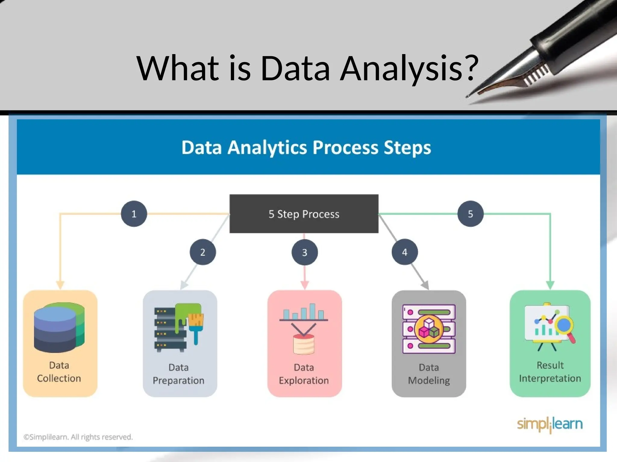
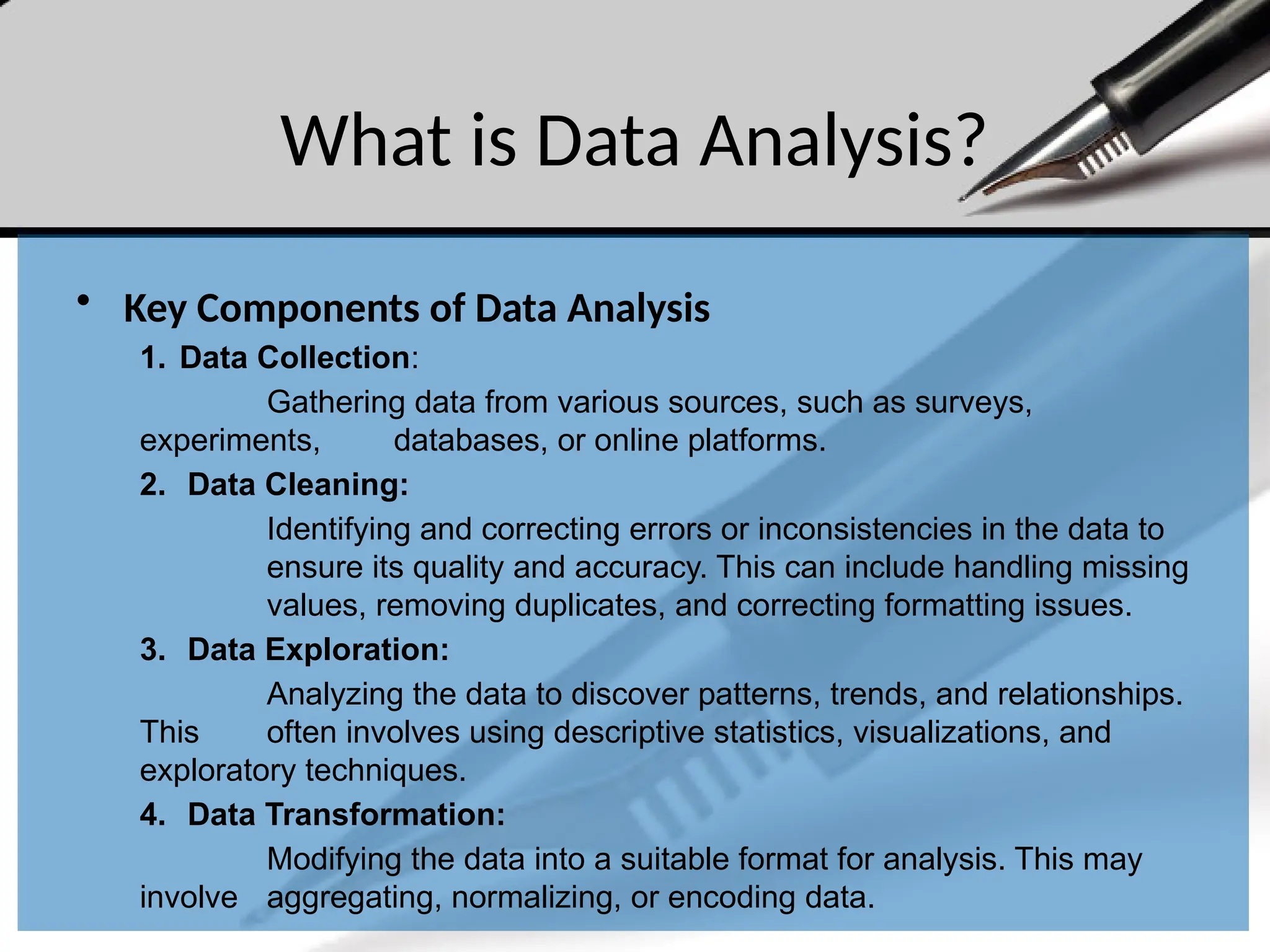
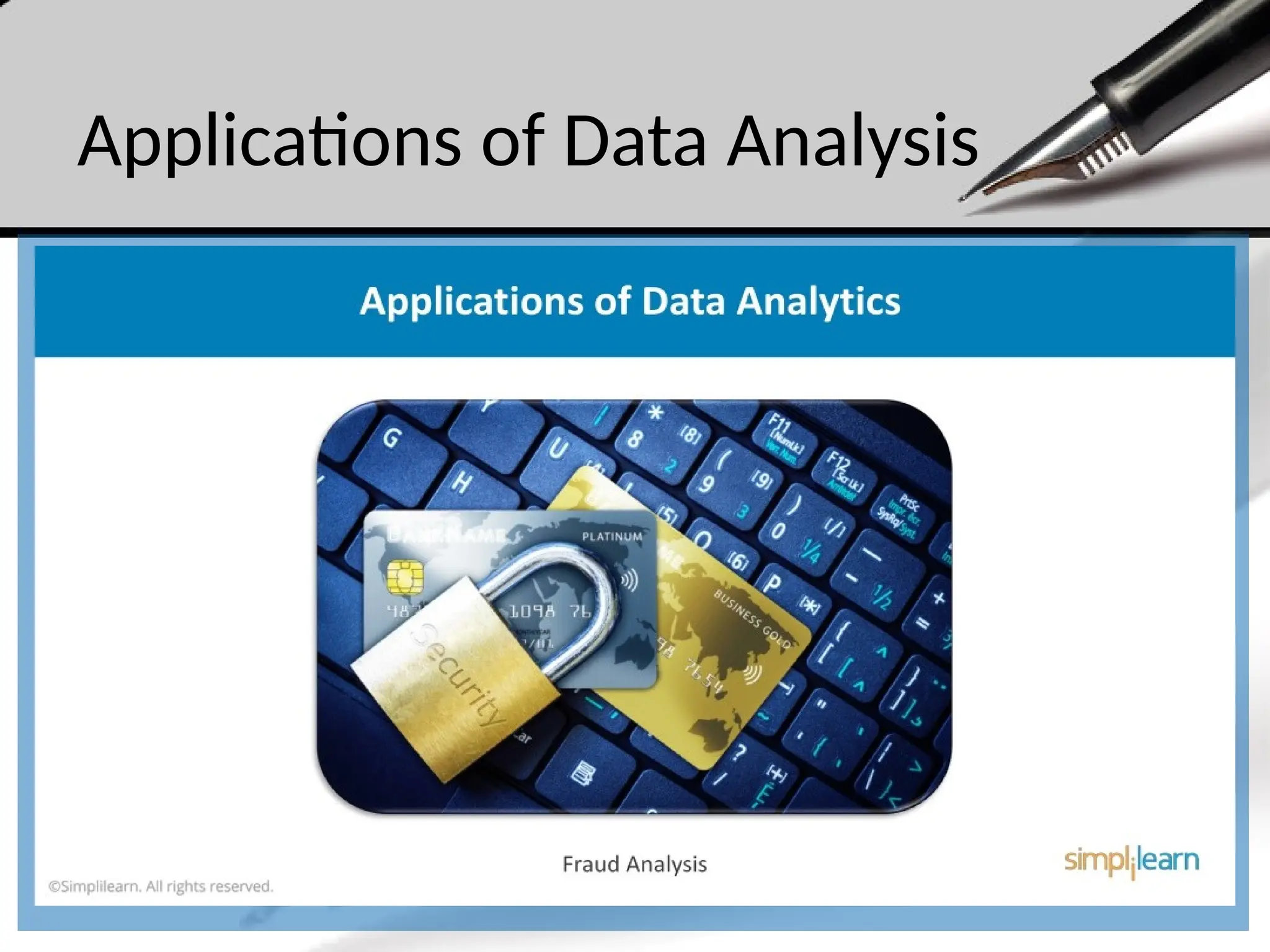
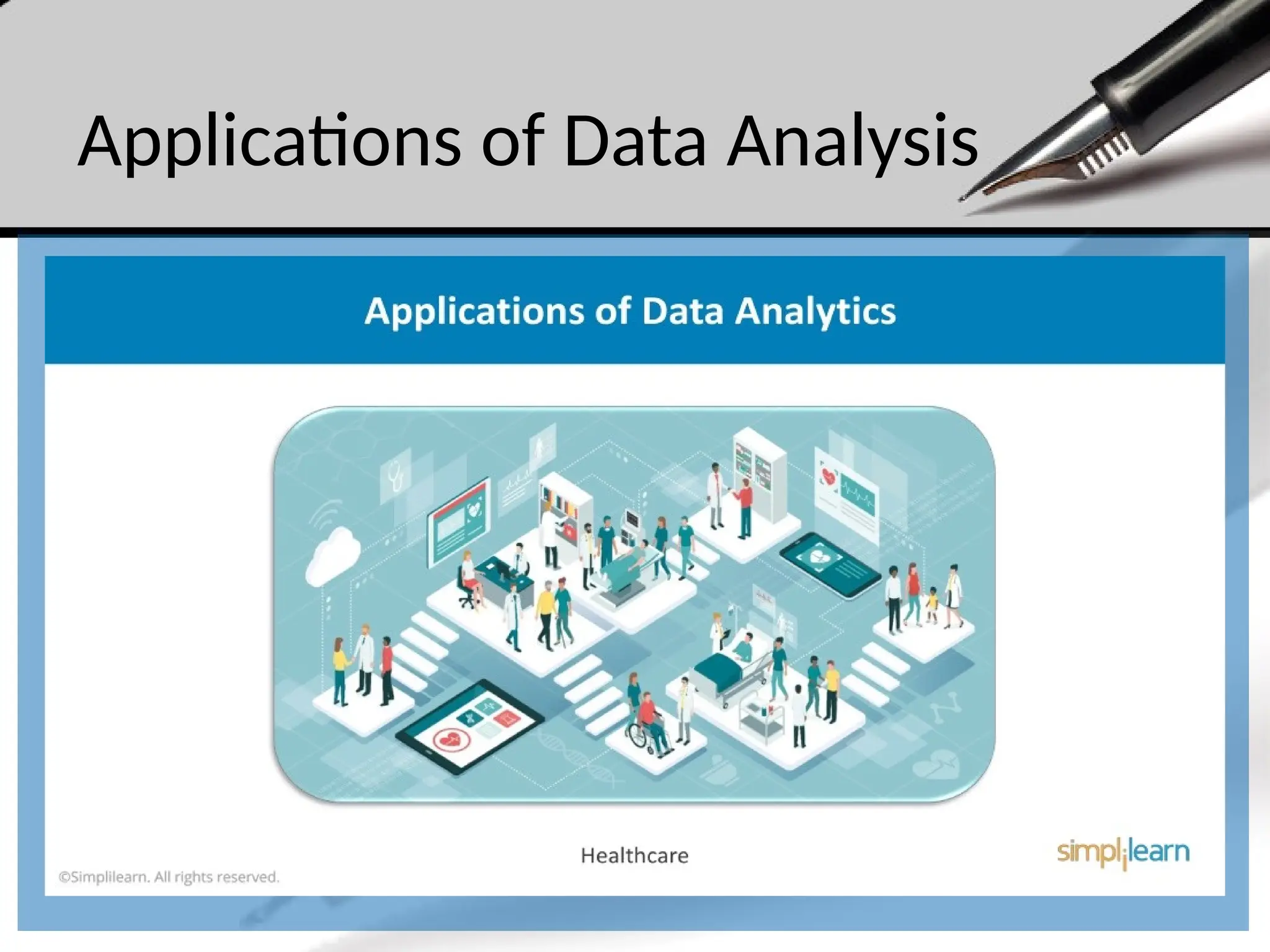
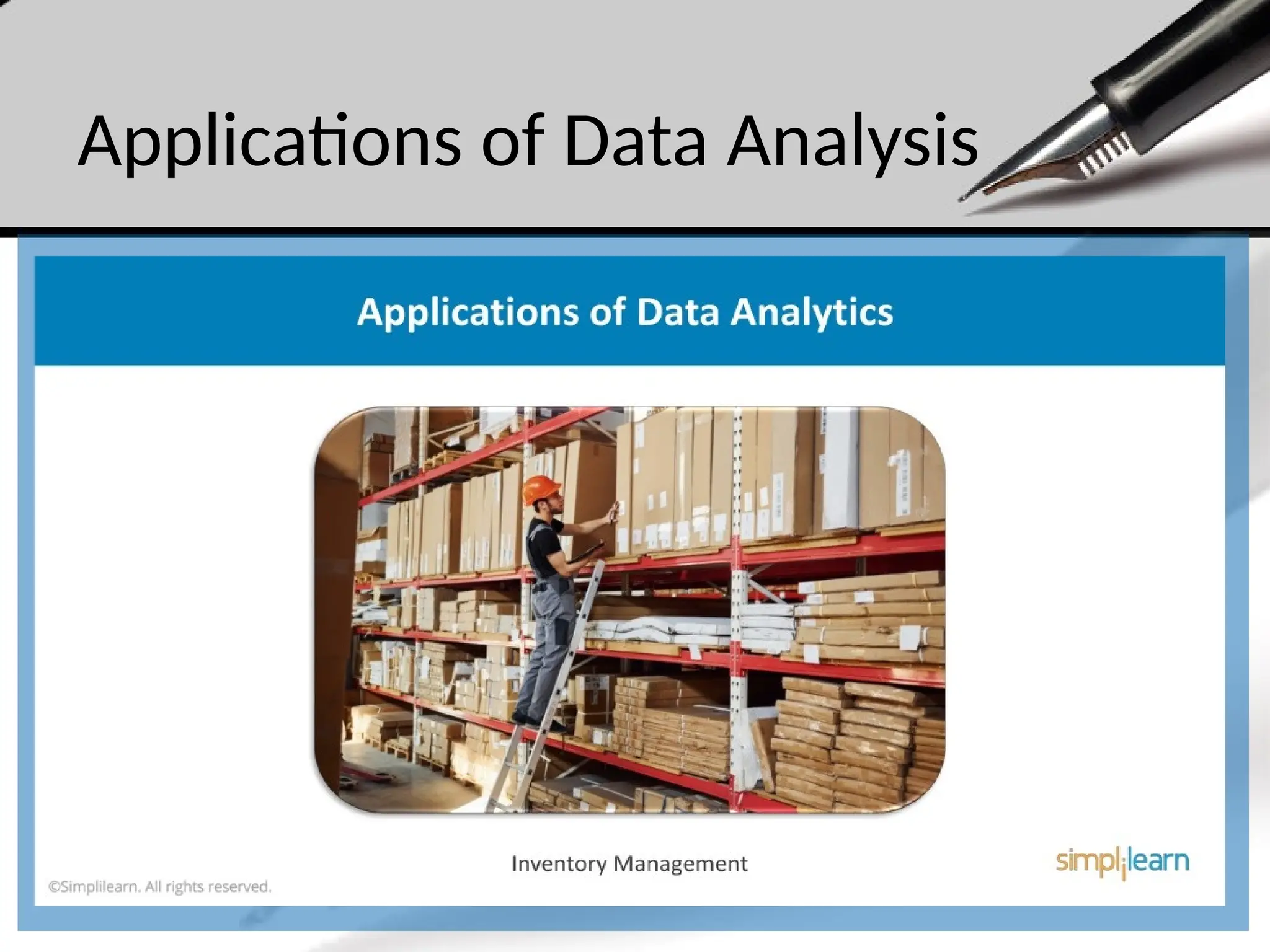
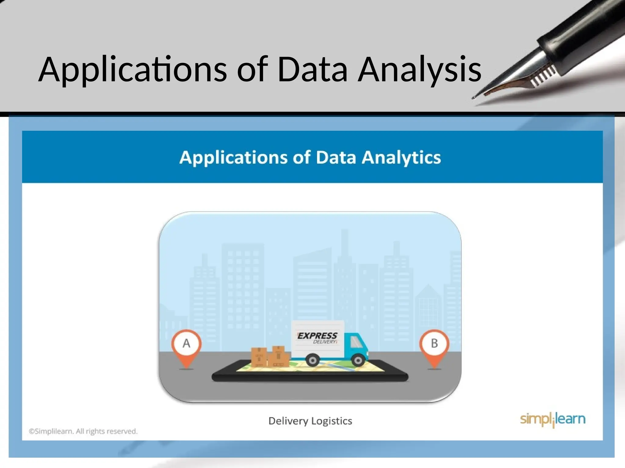
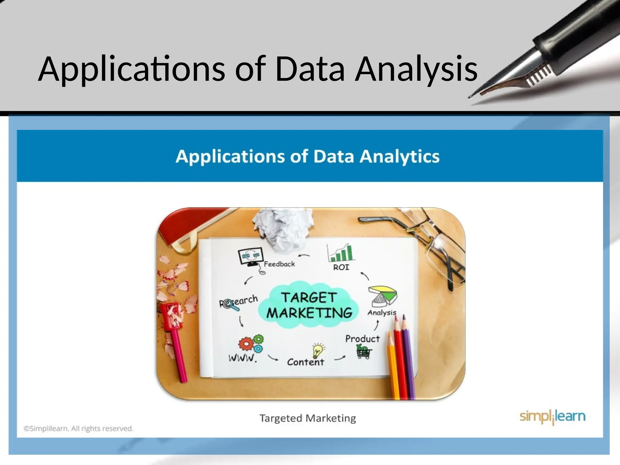

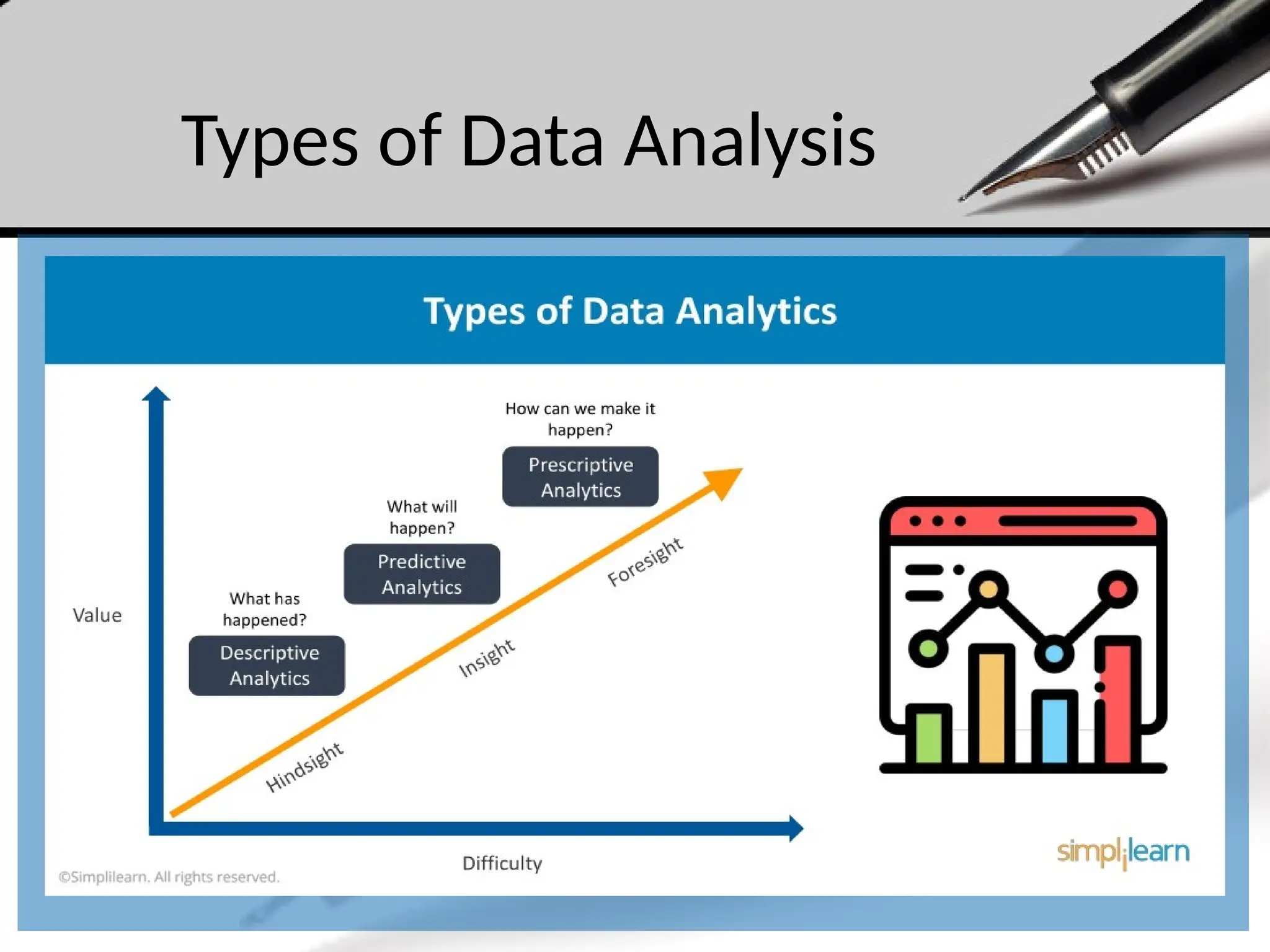
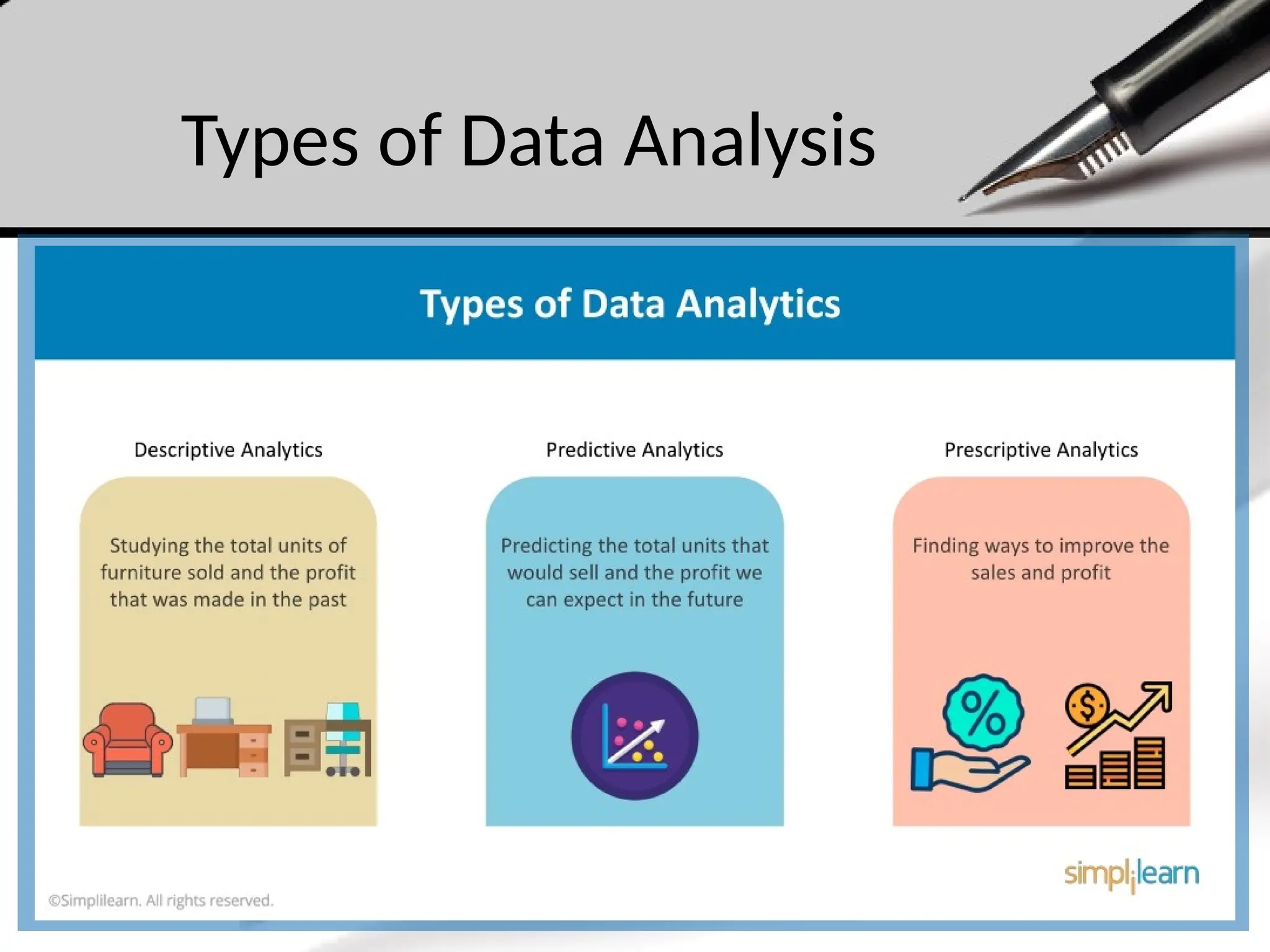
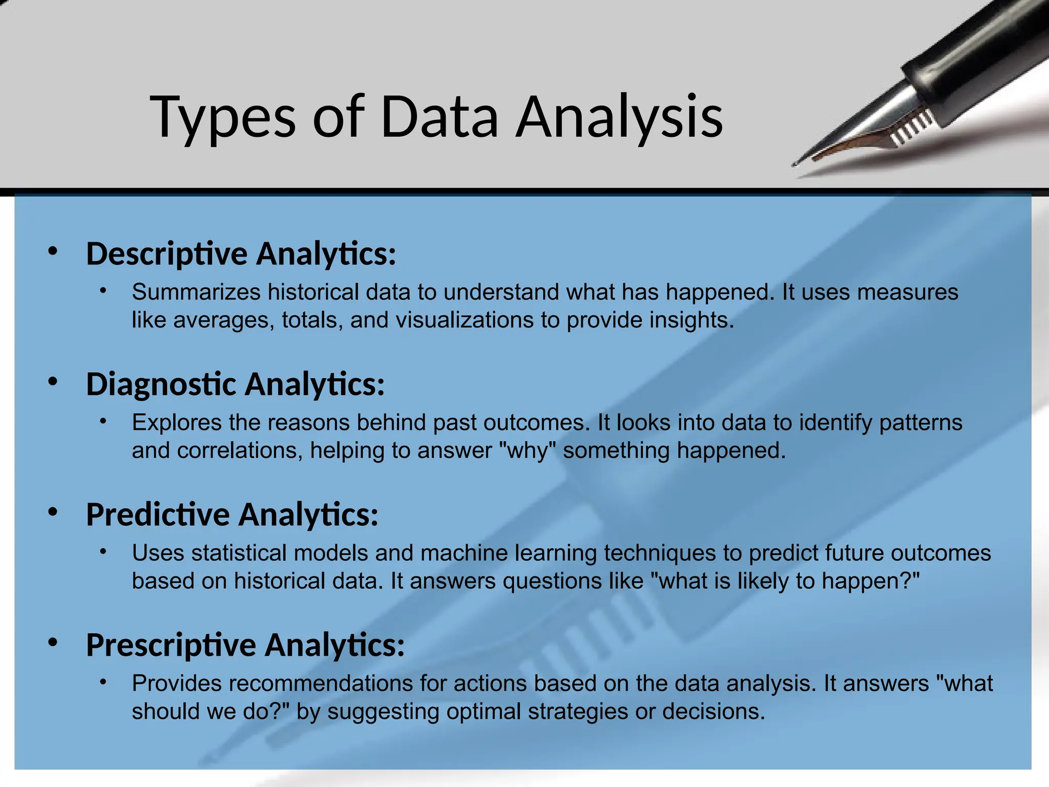
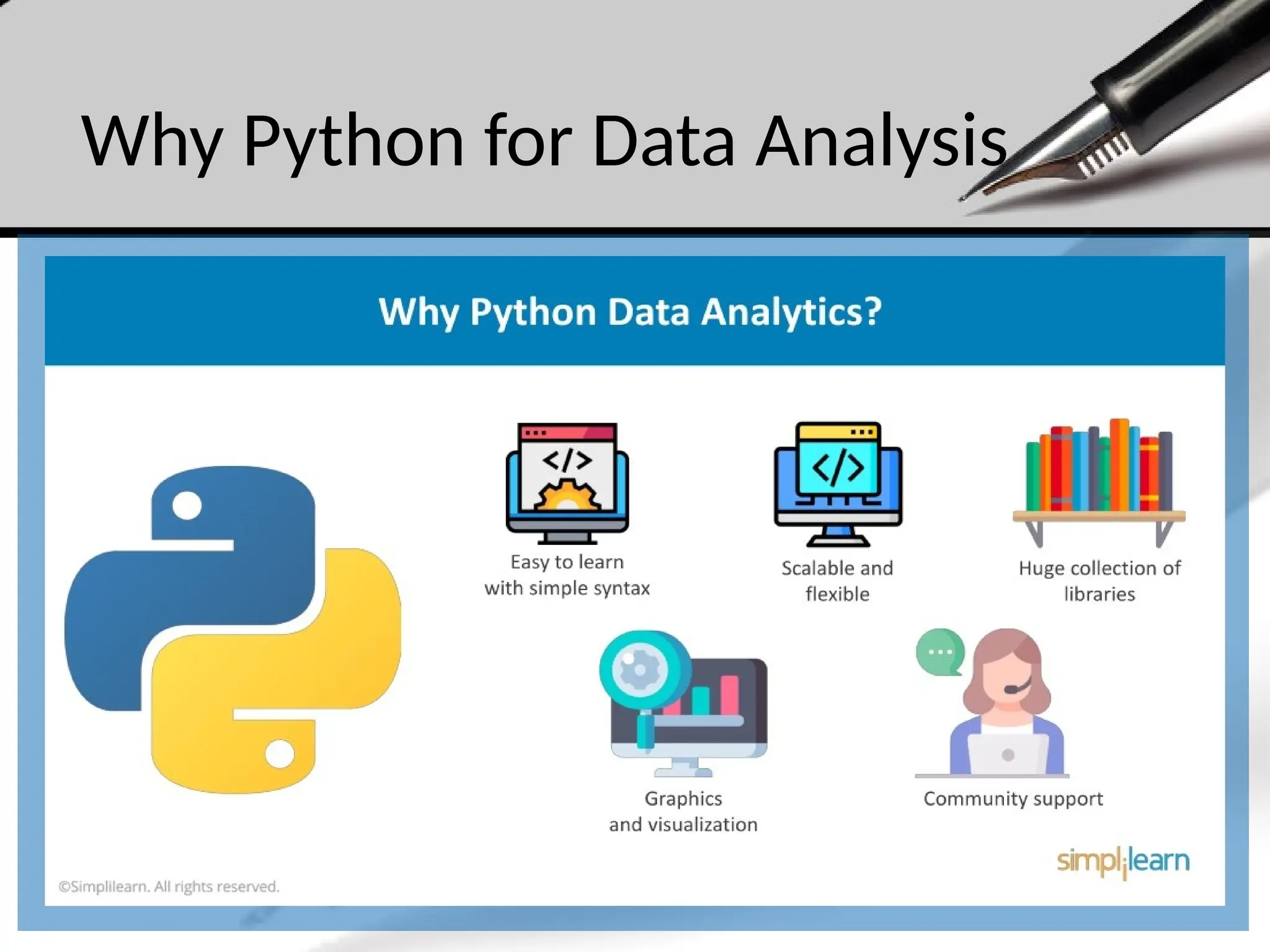

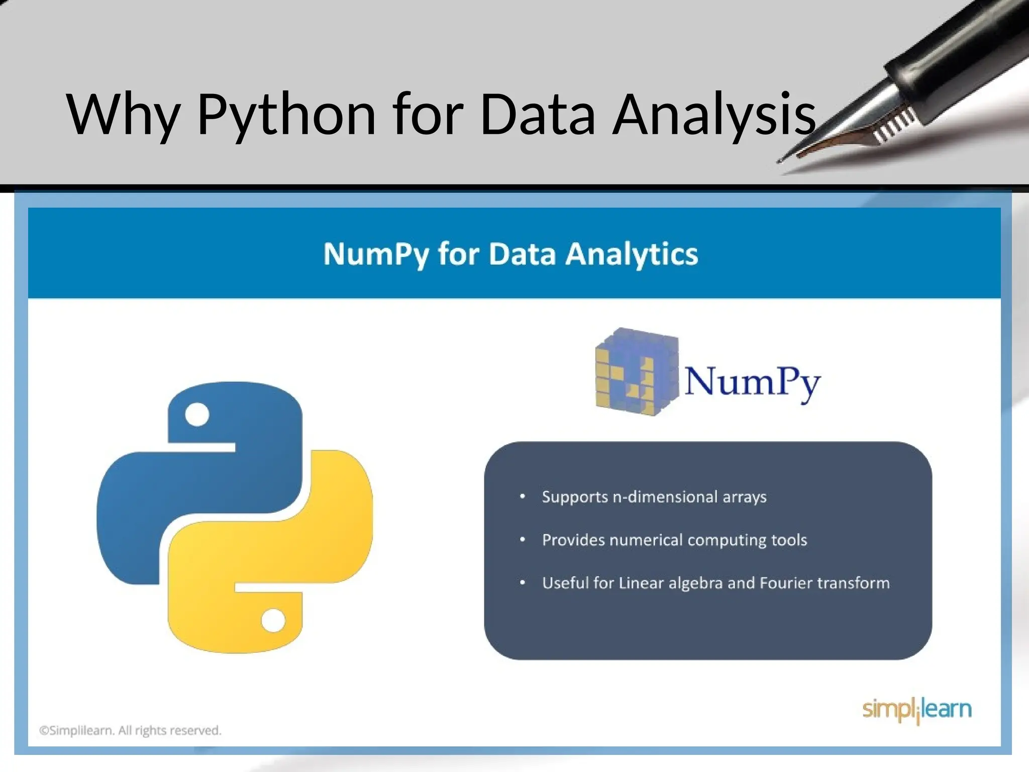
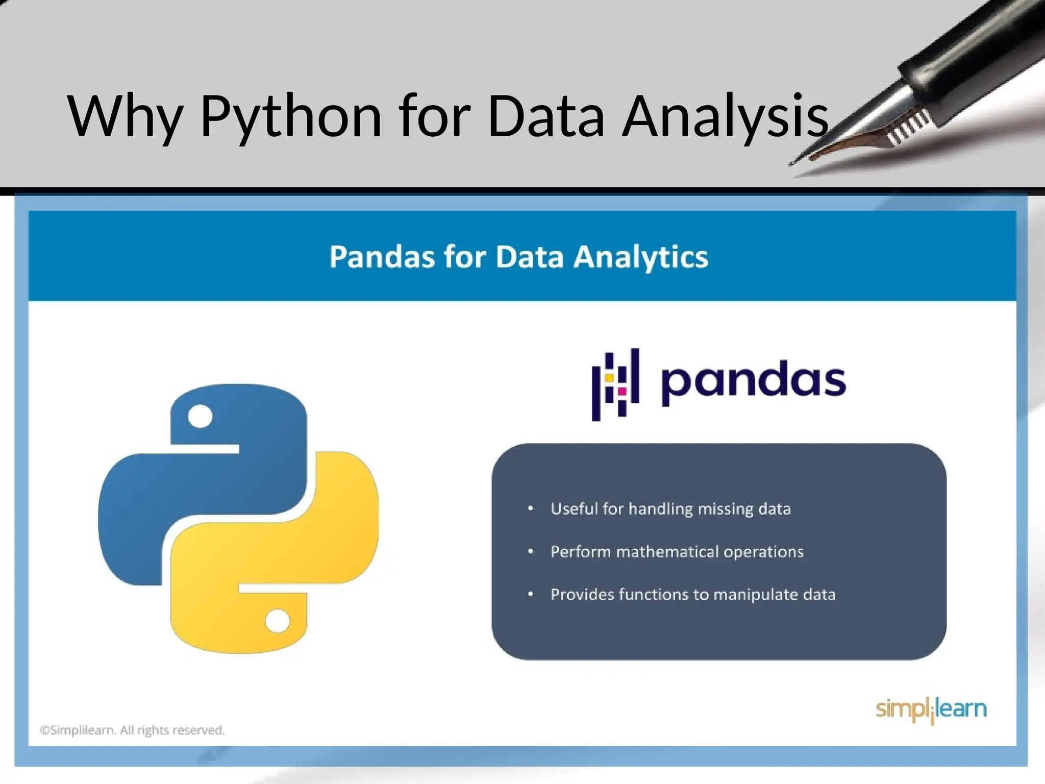
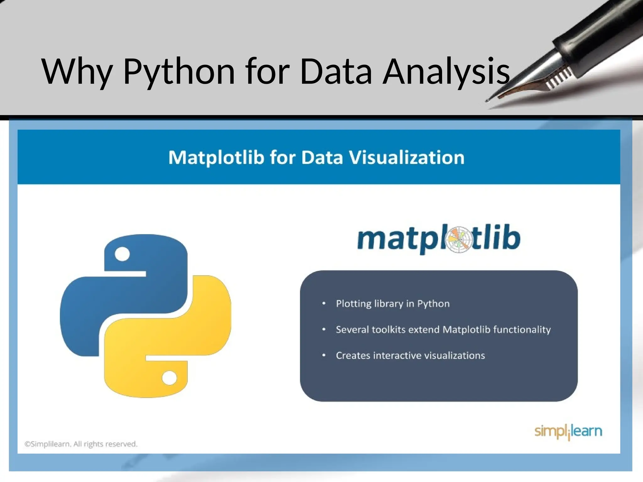
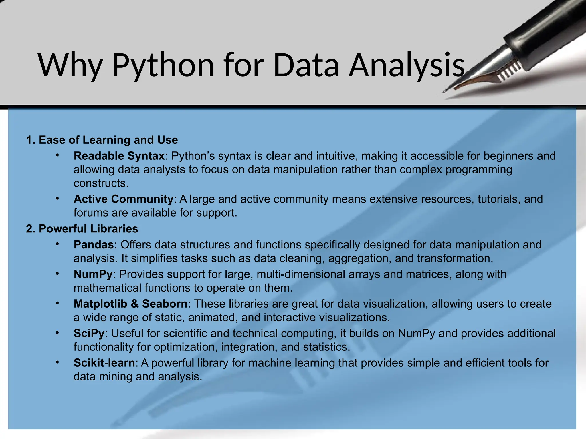
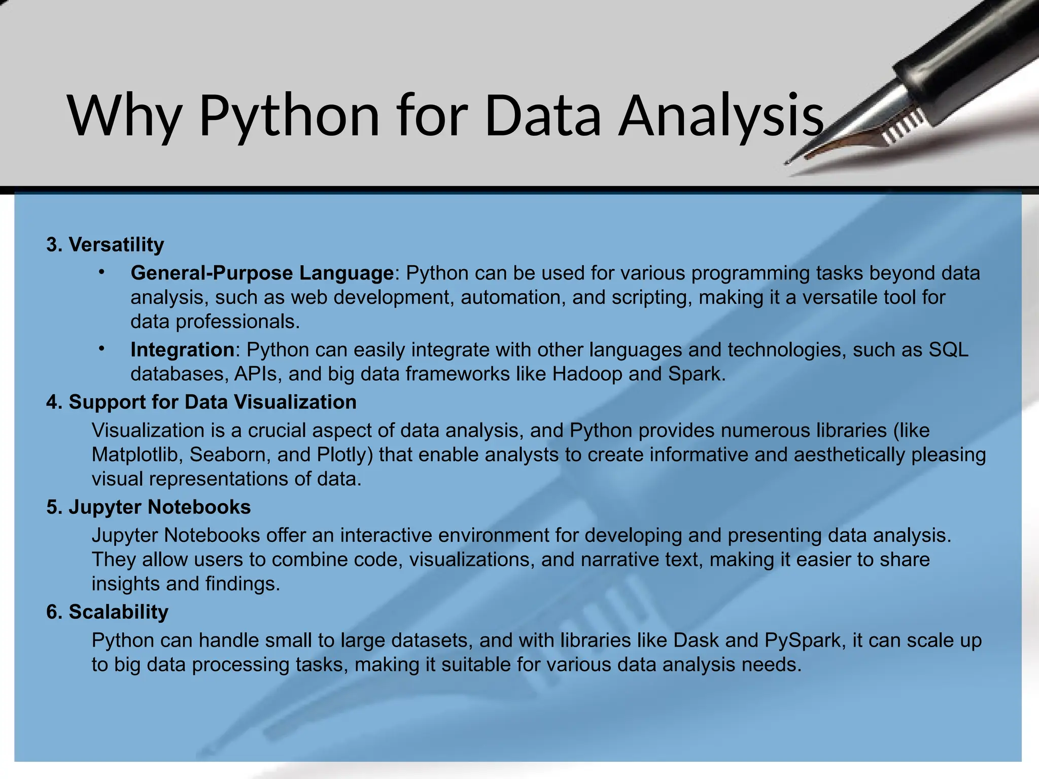
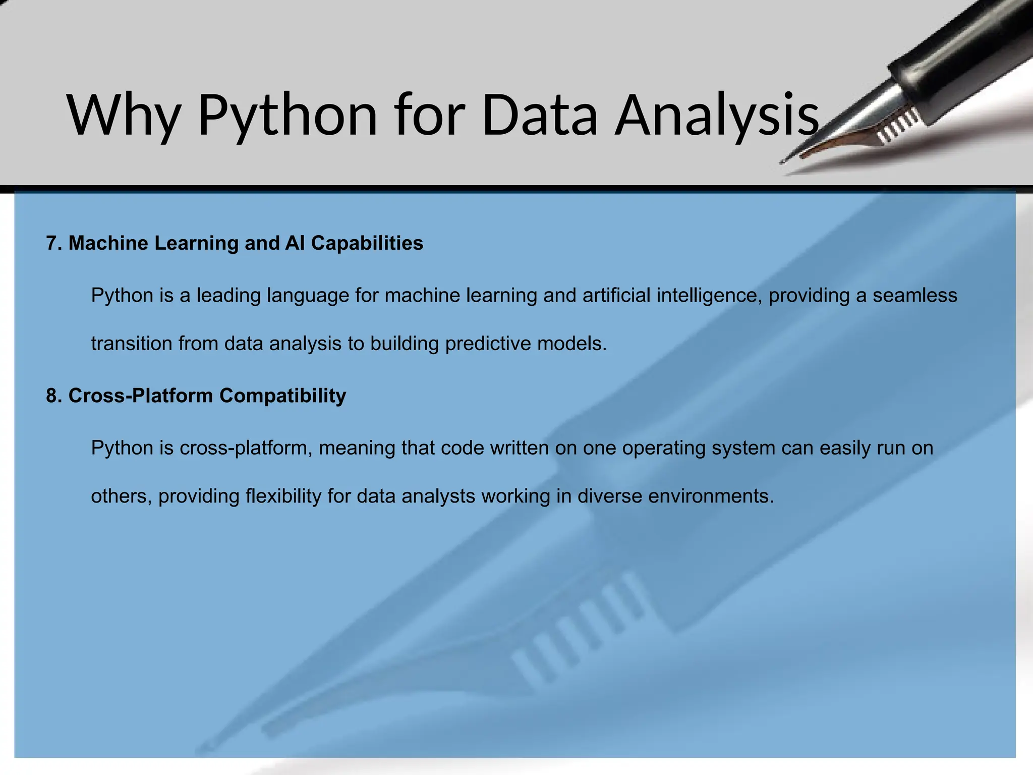
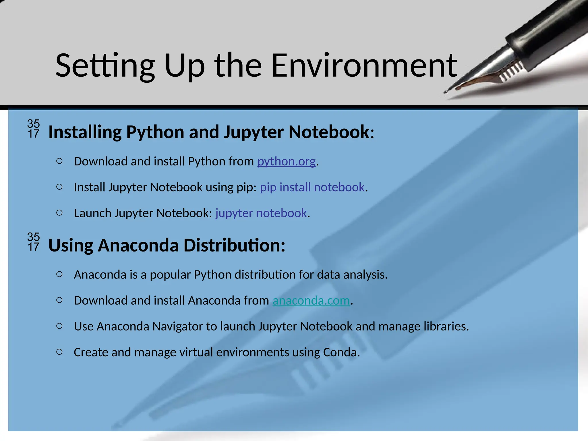
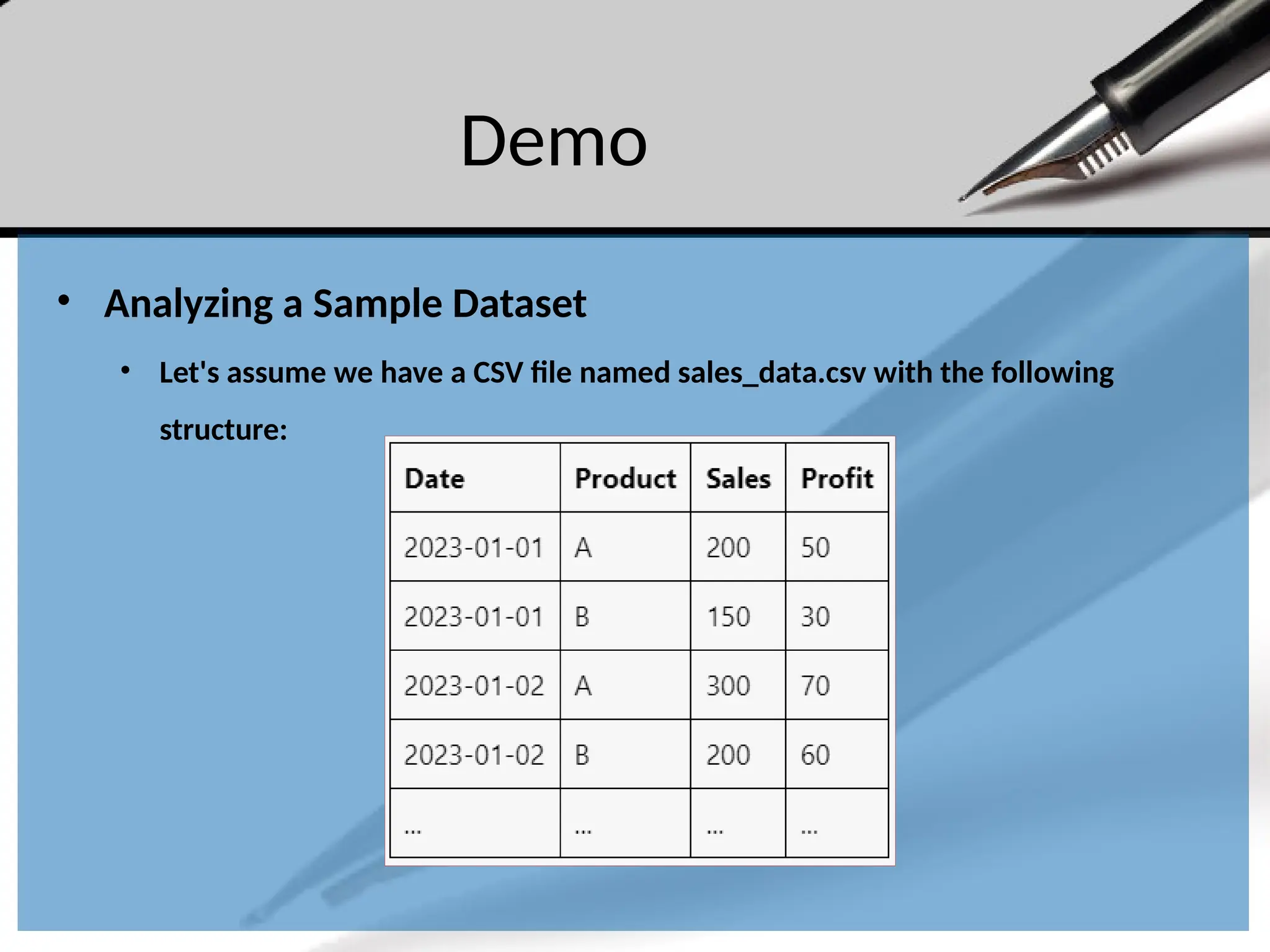
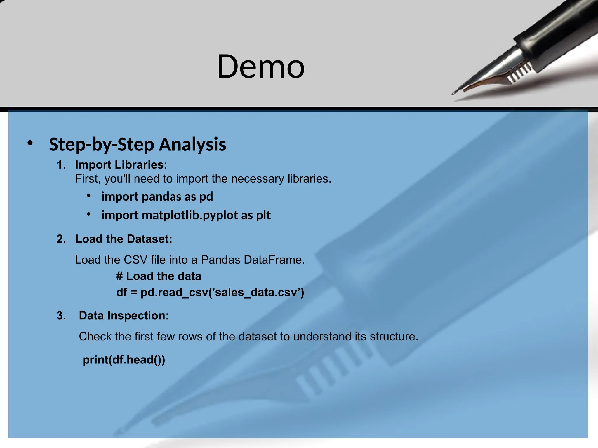
![Demo
• Step-by-Step Analysis
4. Basic Analysis:
Perform some basic analysis to get insights.
# Summary statistics
print(df.describe())
# Total sales and profit per product
total_sales = df.groupby('Product')['Sales'].sum()
total_profit = df.groupby('Product')['Profit'].sum()
print(total_sales)
print(total_profit)](https://image.slidesharecdn.com/dalecture1introduction-250915234621-3db310b6/75/DATA-ANALYSIS_Lecture-1-Introduction-pptx-33-2048.jpg)
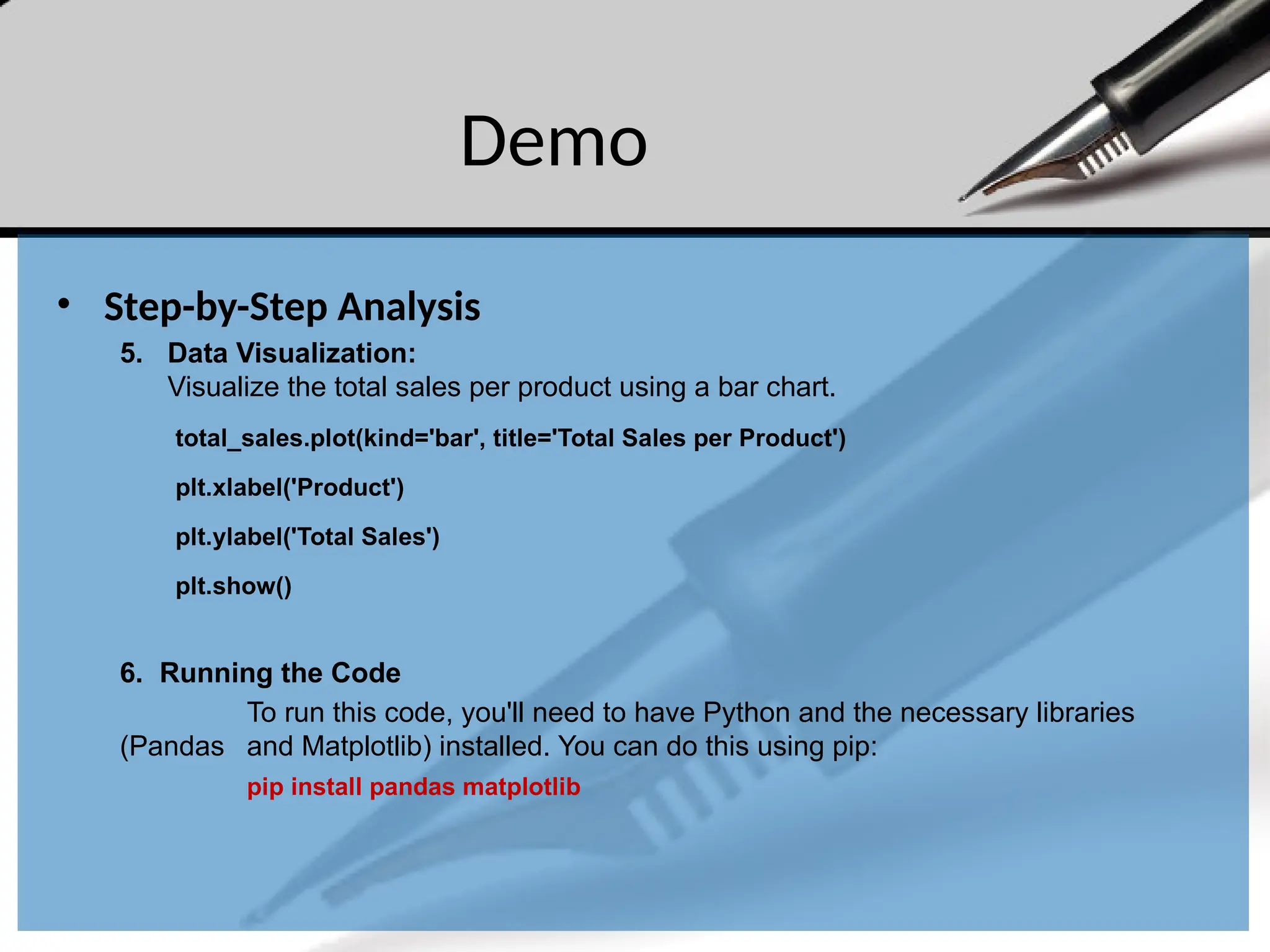
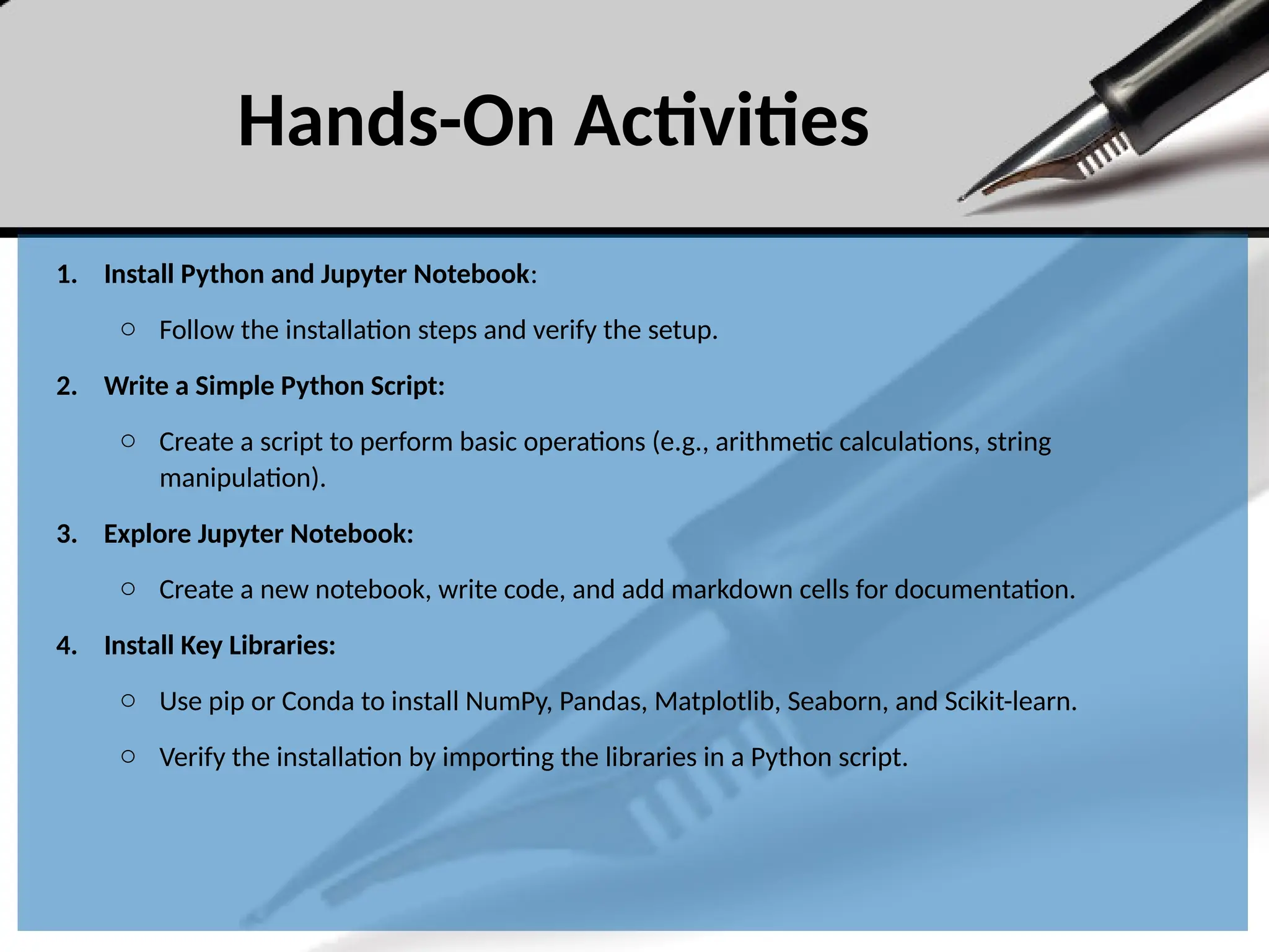


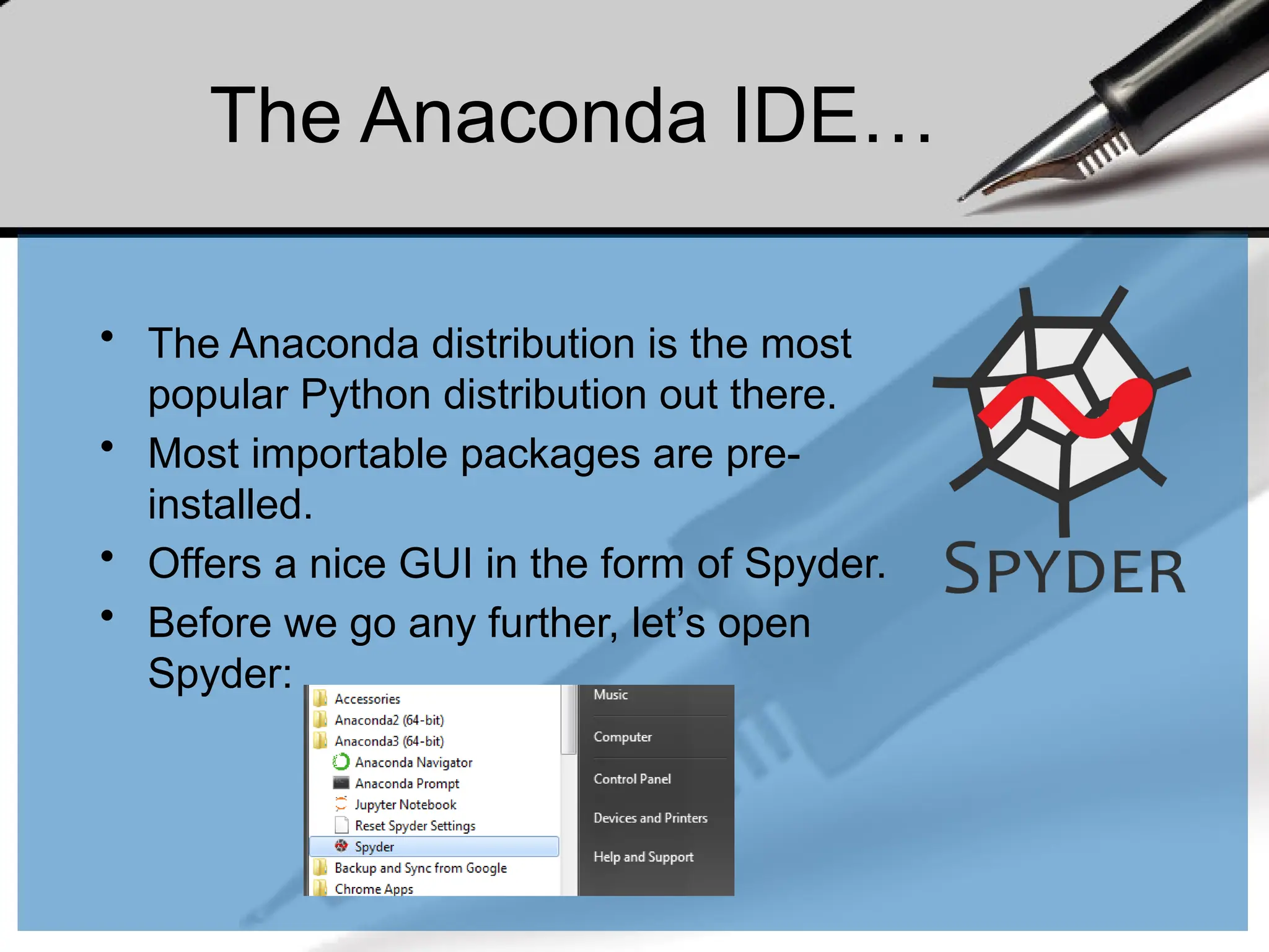
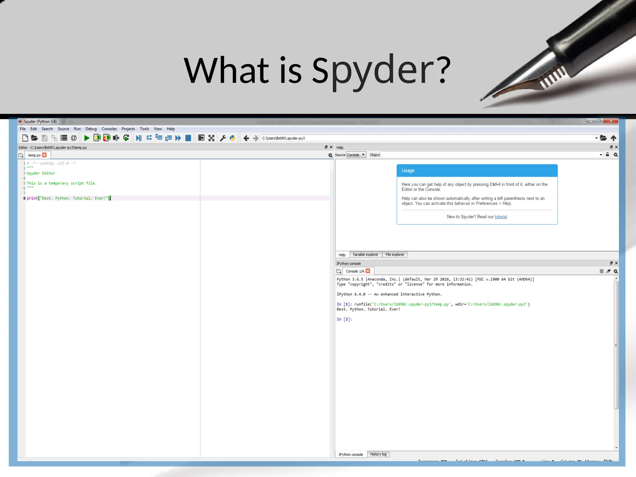
![Variable types
• Integer (int)
• Float (float)
• String (str)
• Boolean (bool)
• Complex (complex)
• […]
• User defined
(classes)
• A variable is assigned using the = operator; i.e:
In: Out:
• Create an integer, float, and string
variable.
• Print these to the screen.
• Play around using different variable
names, etc.
• The print() function is used to print
something to the screen.](https://image.slidesharecdn.com/dalecture1introduction-250915234621-3db310b6/75/DATA-ANALYSIS_Lecture-1-Introduction-pptx-46-2048.jpg)
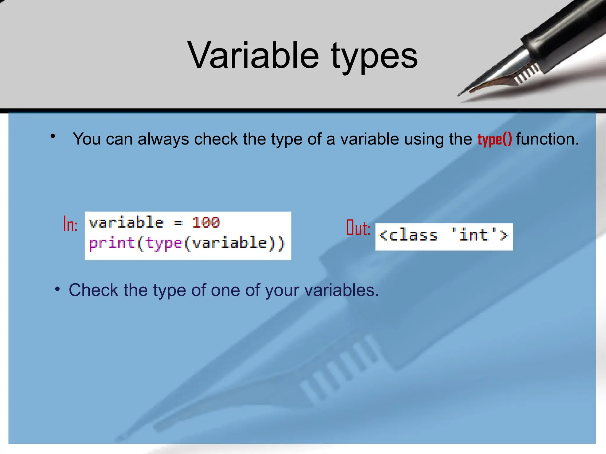
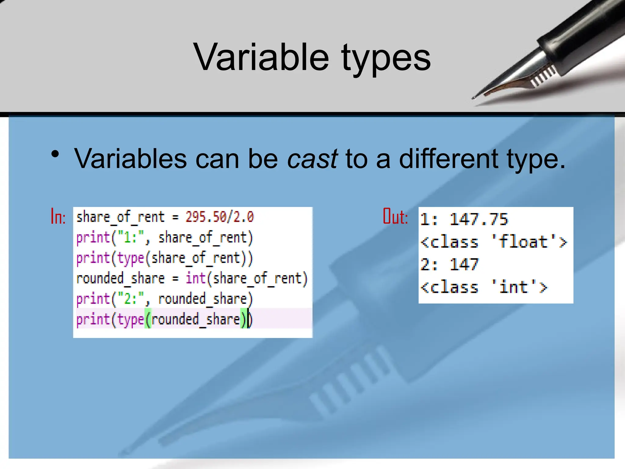
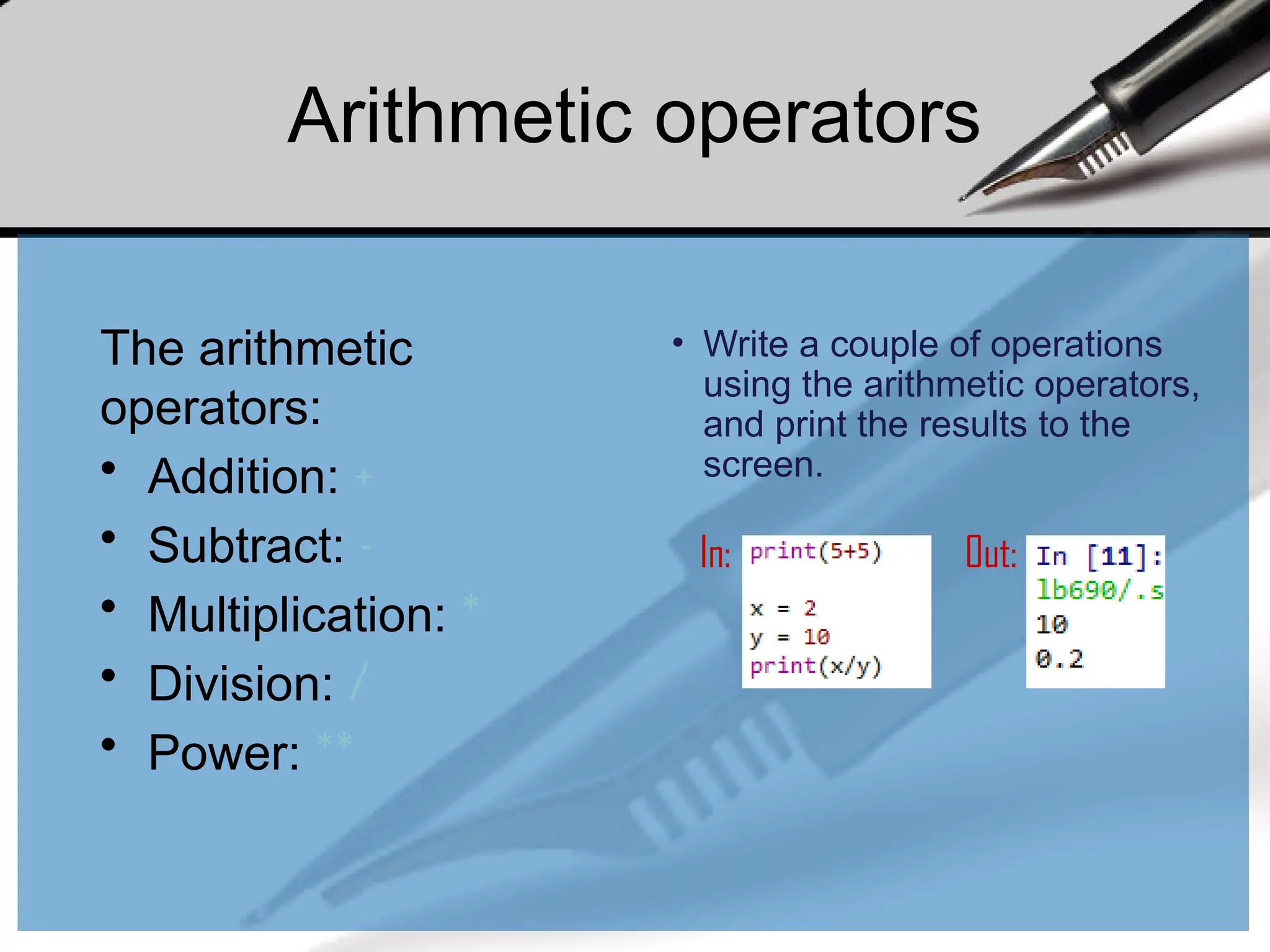
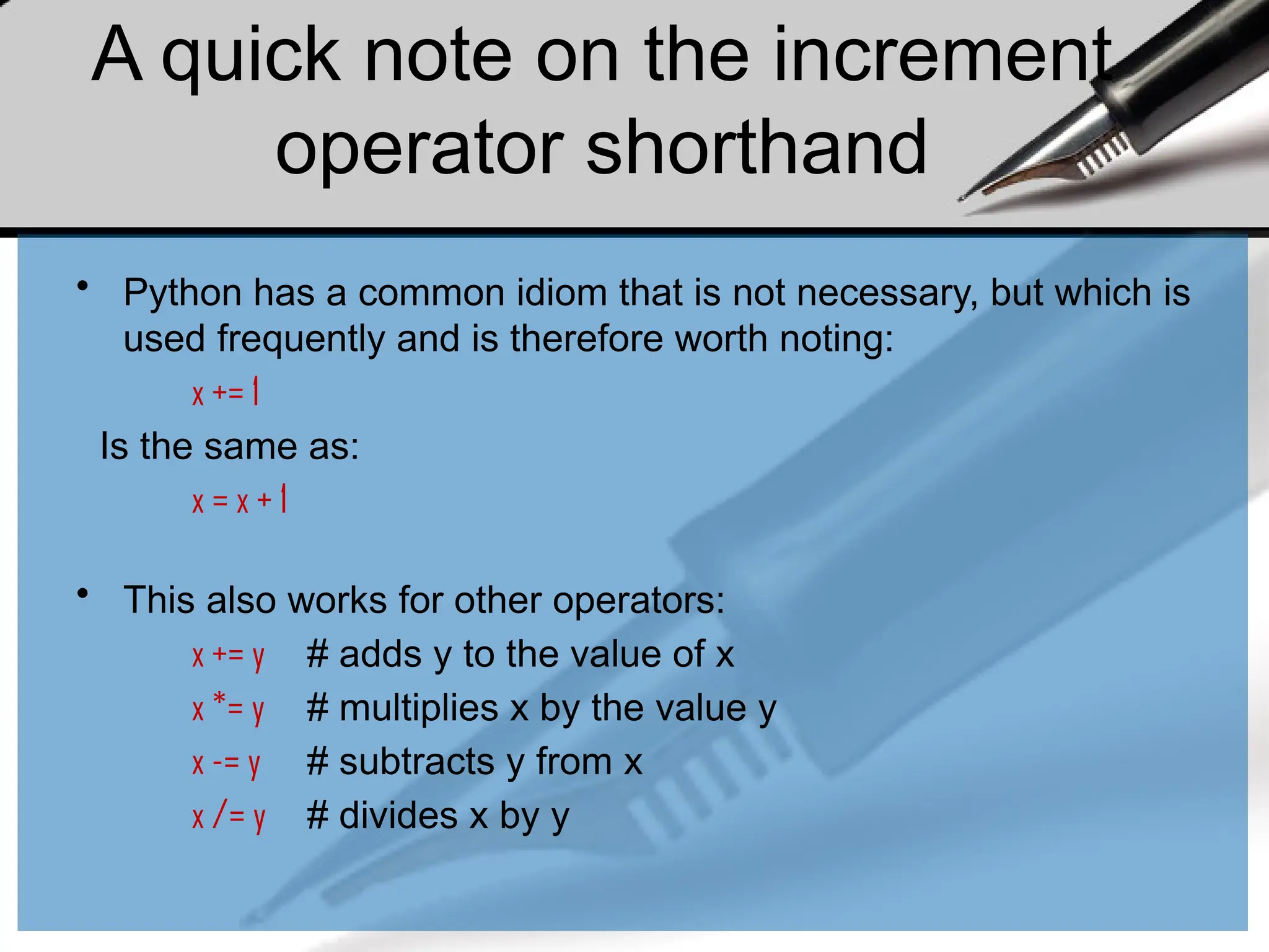

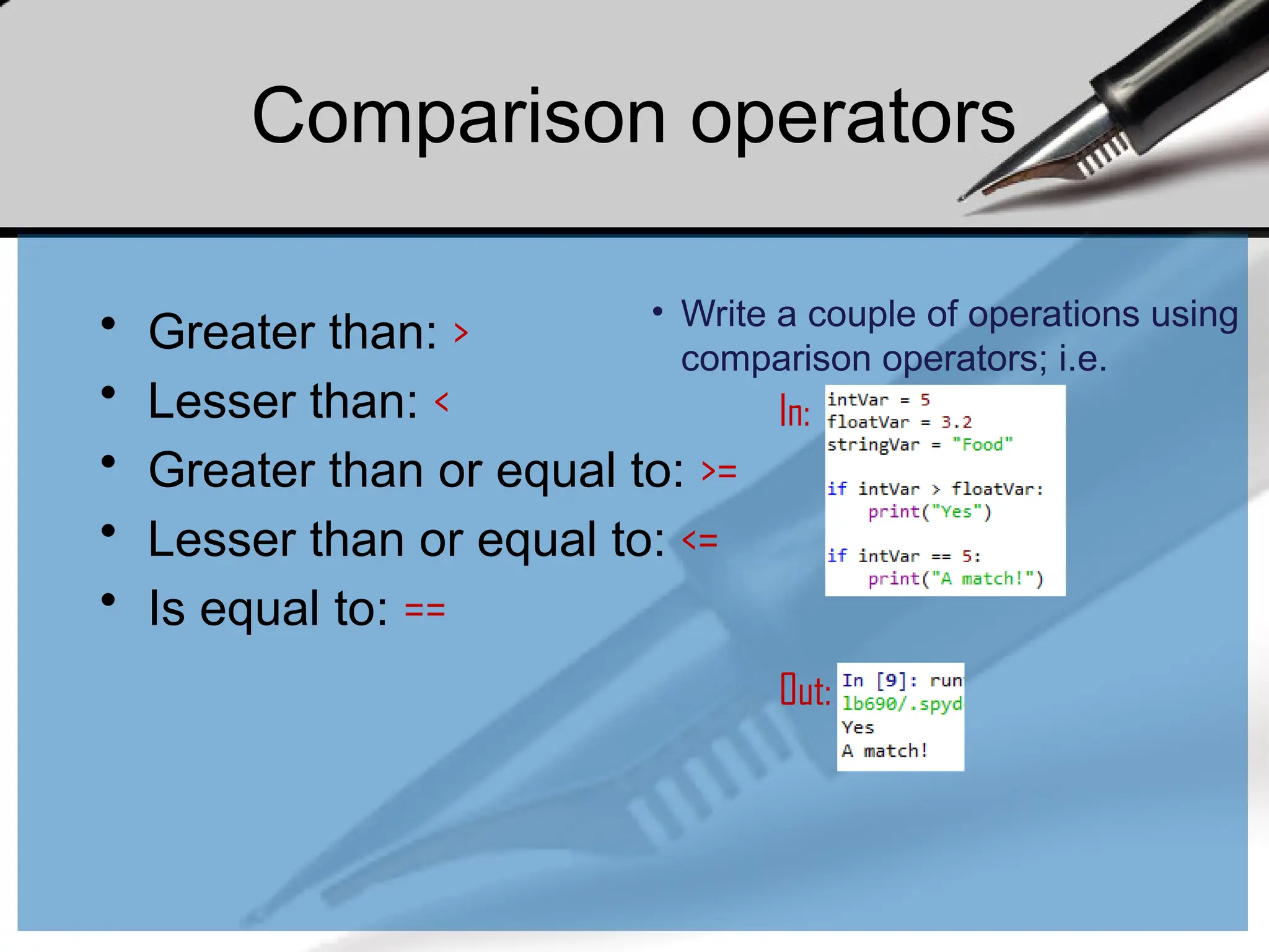
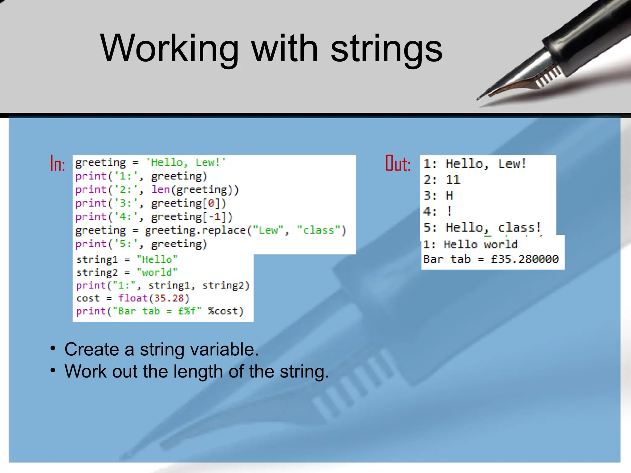
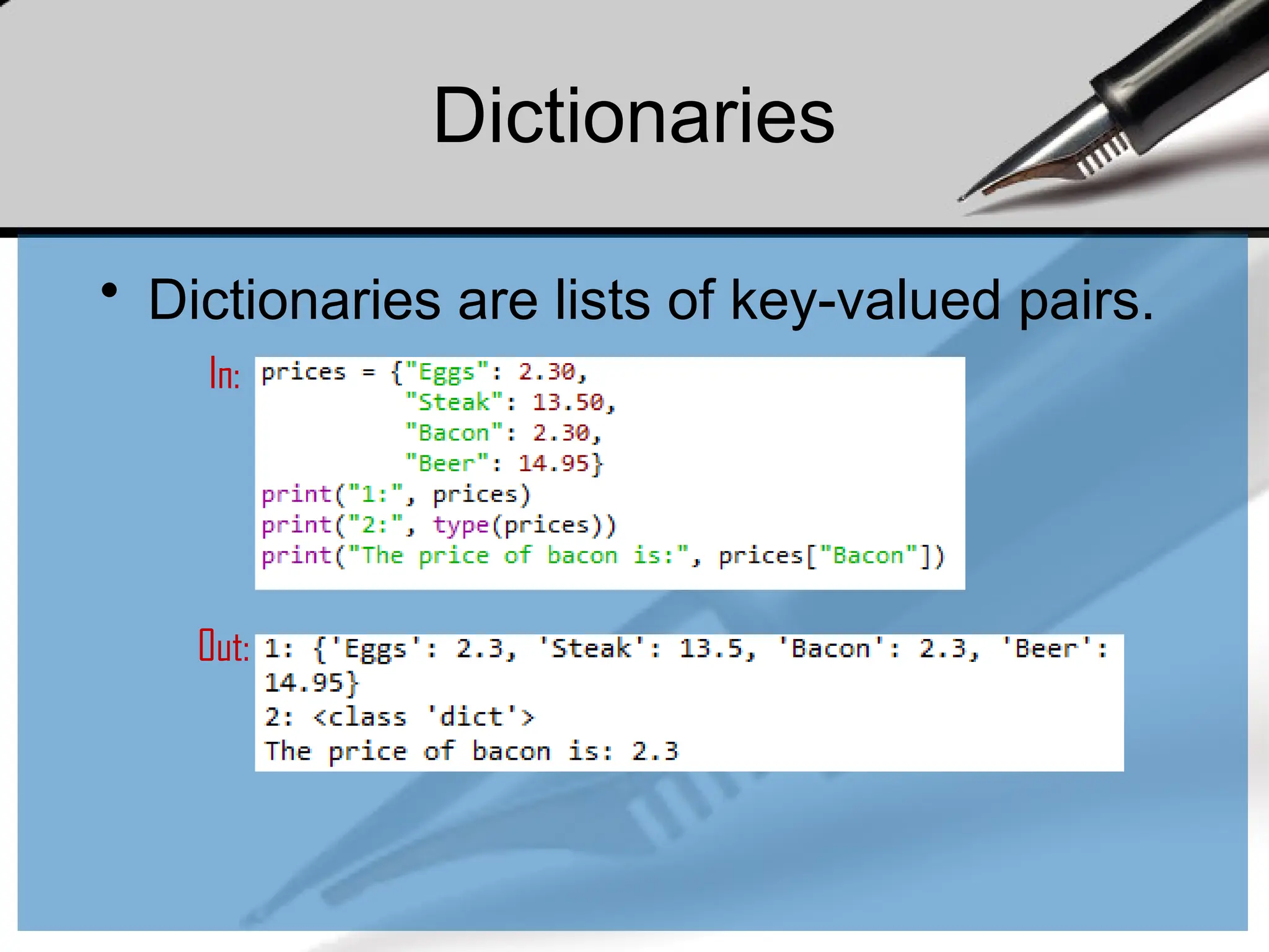
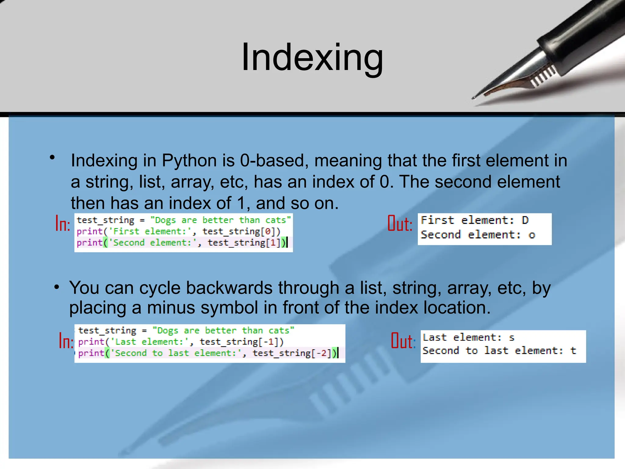
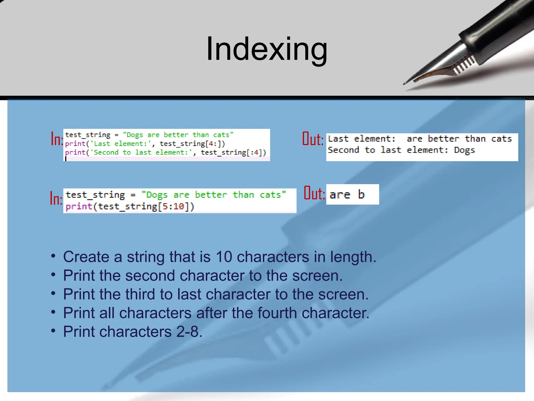
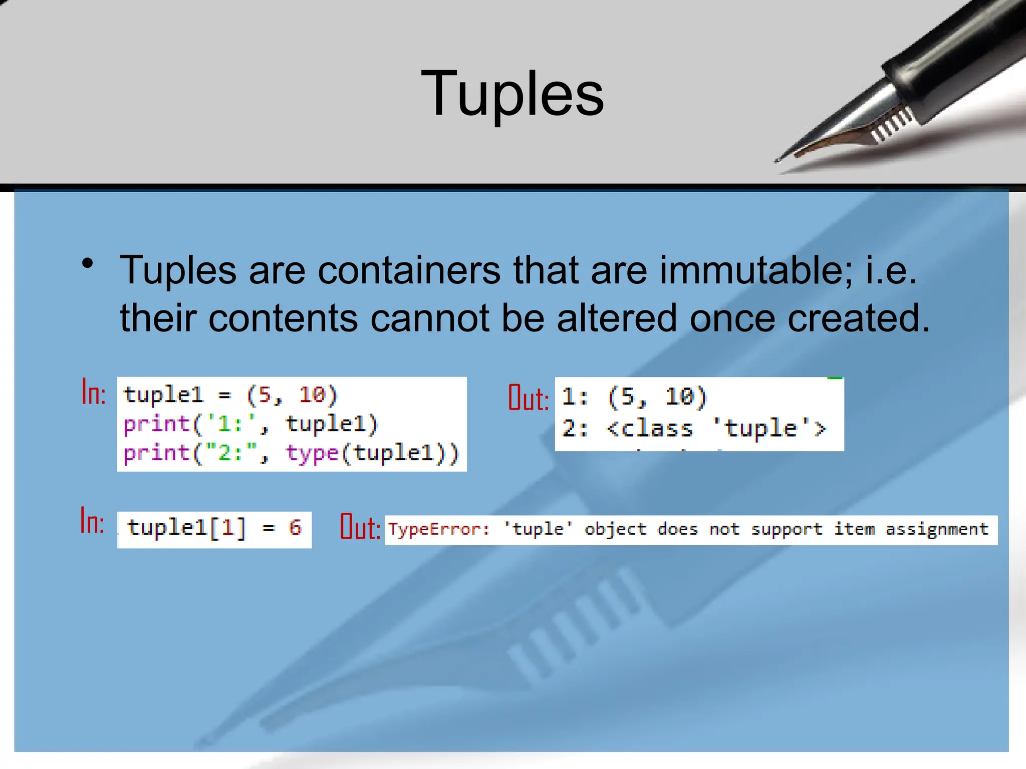
![Lists
• Lists are essentially containers of arbitrary
type.
• They are probably the container that you will
use most frequently.
• The elements of a list can be of different
types.
• The difference between tuples and lists is in
performance; it is much faster to ‘grab’ an
element stored in a tuple, but lists are much
more versatile.
• Note that lists are denoted by [] and not the ()
used by tuples.
In:
Out:
• Create a list and populate it with some elements.](https://image.slidesharecdn.com/dalecture1introduction-250915234621-3db310b6/75/DATA-ANALYSIS_Lecture-1-Introduction-pptx-58-2048.jpg)
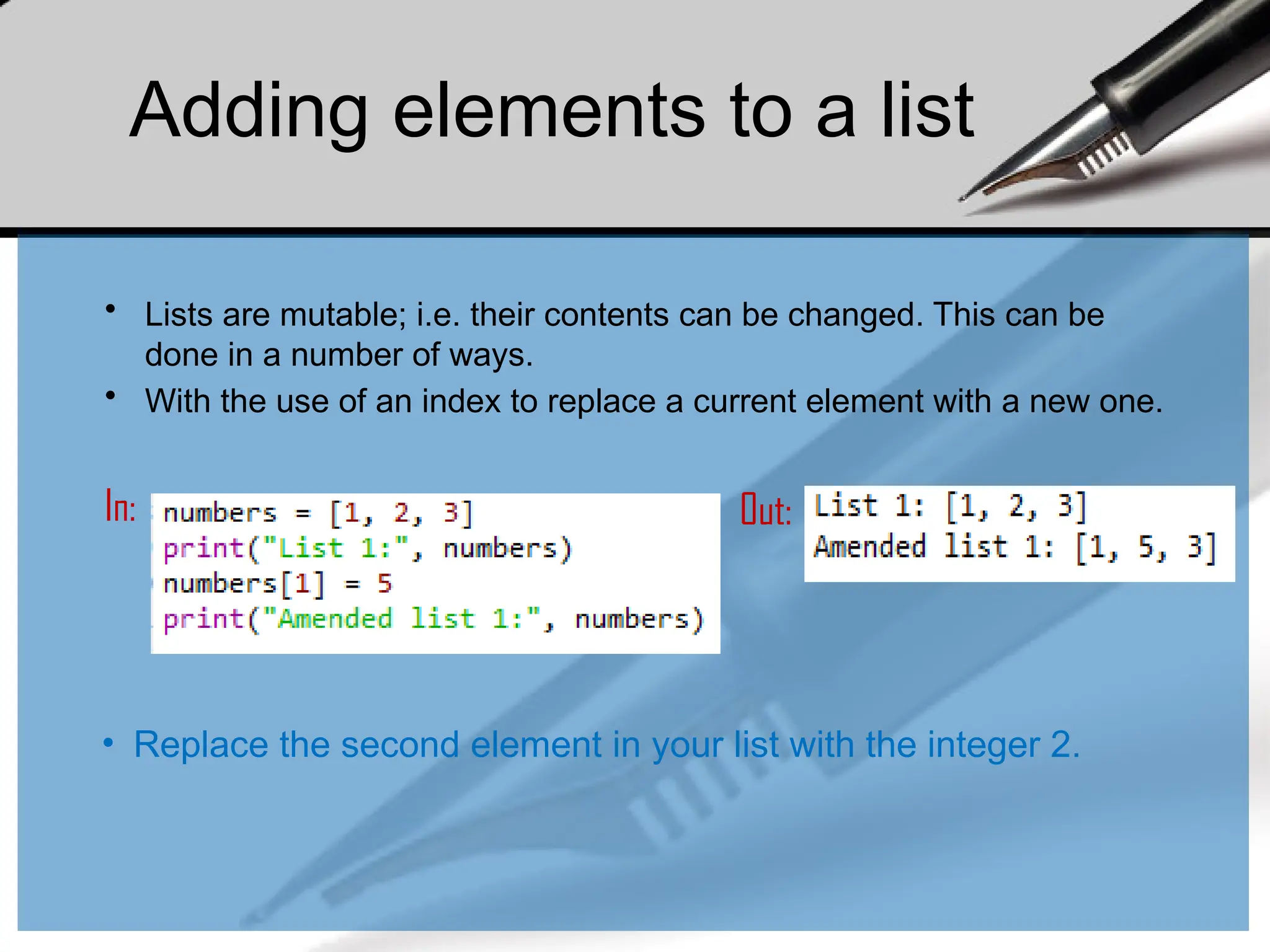
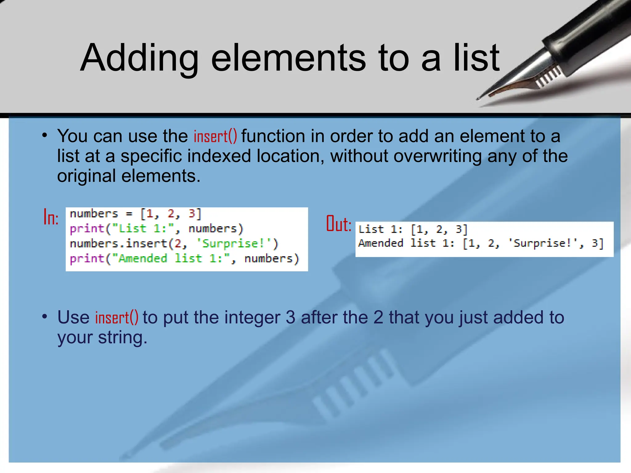
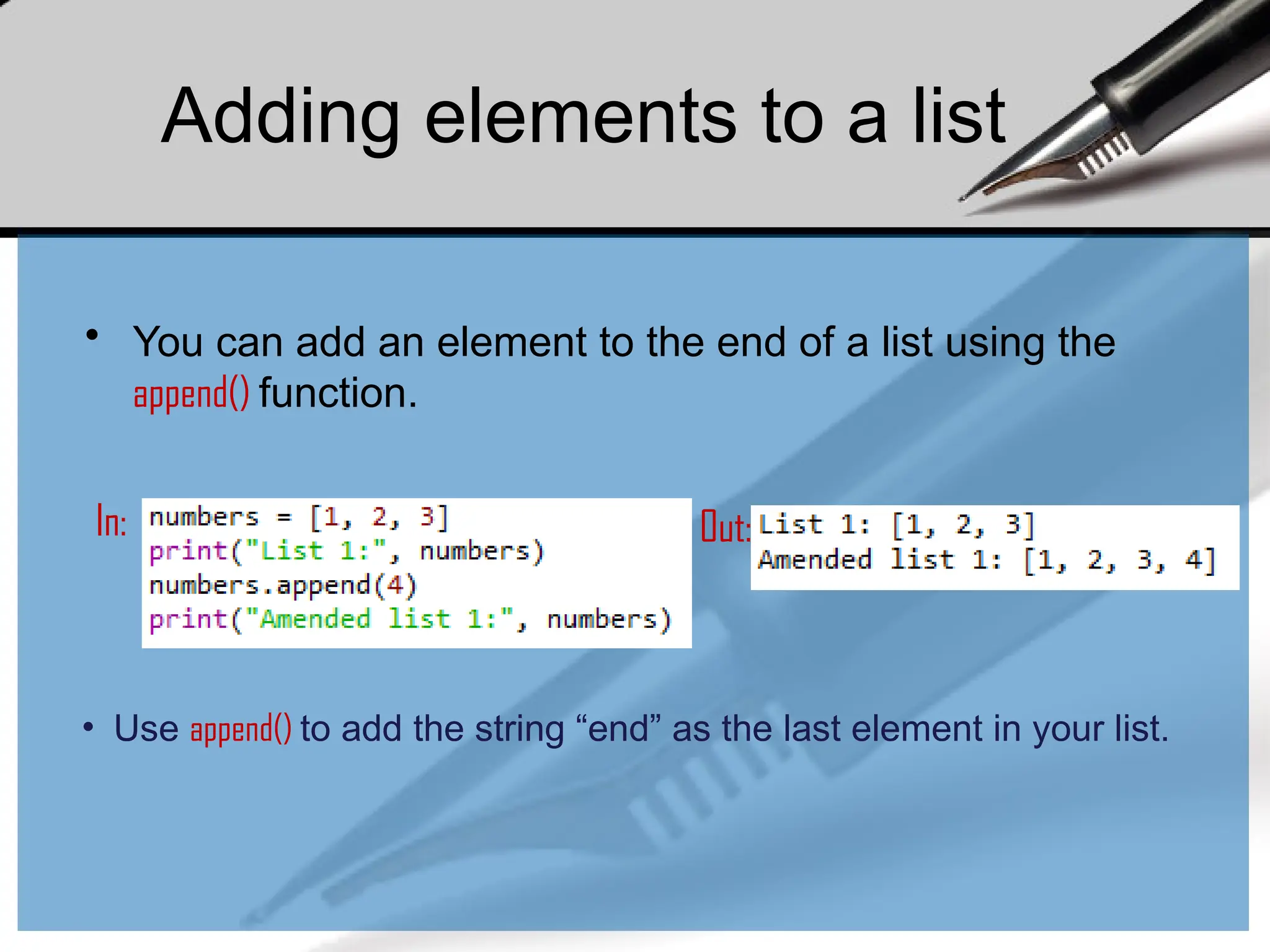
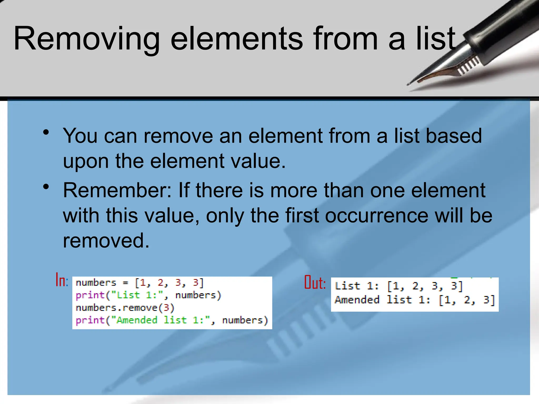
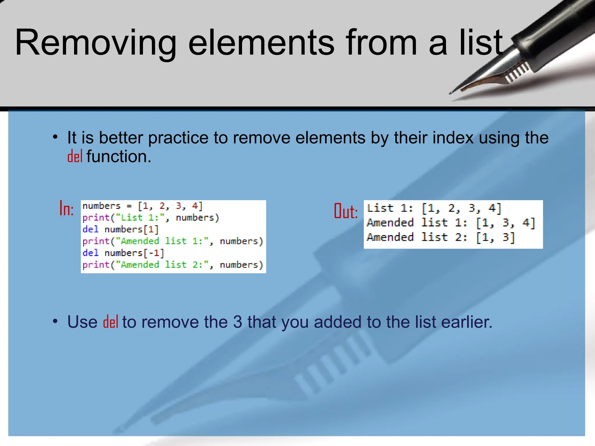
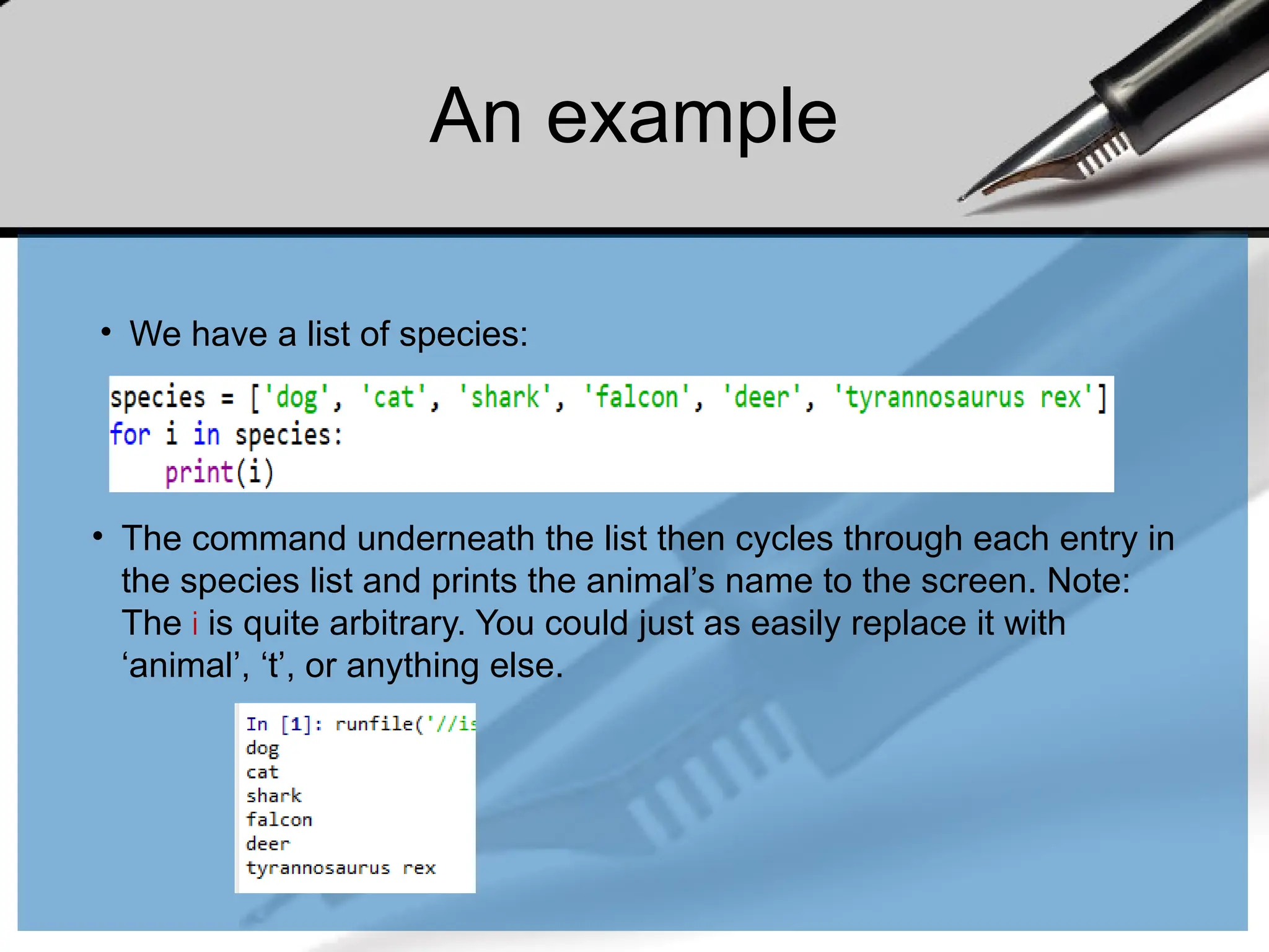
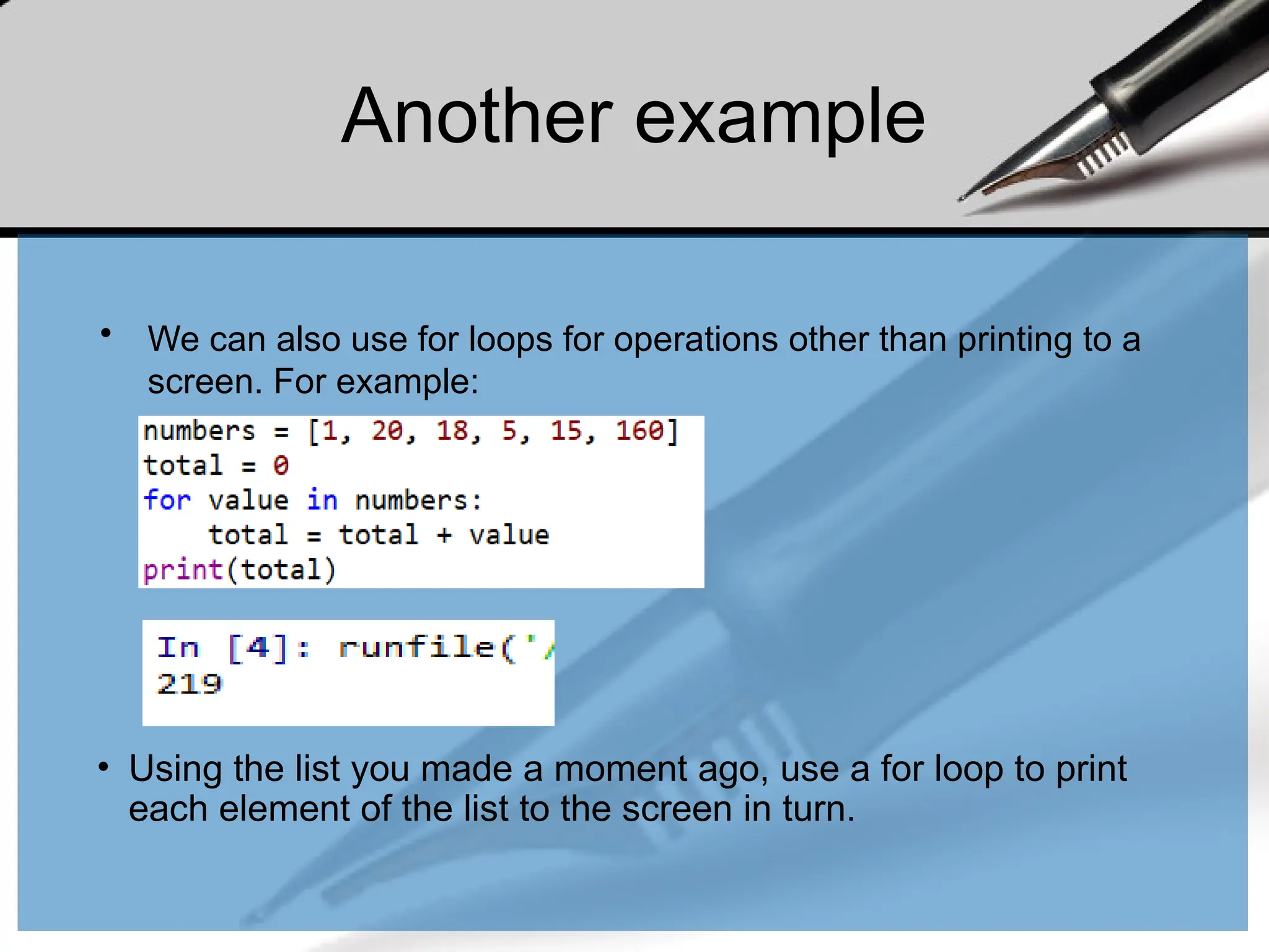
![The range() function
• The range() function generates a list of numbers, which is generally used to
iterate over within for loops.
• The range() function has two sets of parameters to follow:
range(stop)
stop: Number of integers
(whole numbers) to generate,
starting from zero. i.e:
range([start], stop[, step])
start: Starting number of the sequence.
stop: Generate numbers up to, but not including this
number.
step: Difference between each number in the
sequence. i.e.:
Note:
• All parameters must be integers.
• Parameters can be positive or negative.
• The range() function (and Python in general) is 0-index based, meaning list indexes start at 0,
not 1. eg. The syntax to access the first element of a list is mylist[0]. Therefore the last
integer generated by range() is up to, but not including, stop.](https://image.slidesharecdn.com/dalecture1introduction-250915234621-3db310b6/75/DATA-ANALYSIS_Lecture-1-Introduction-pptx-67-2048.jpg)
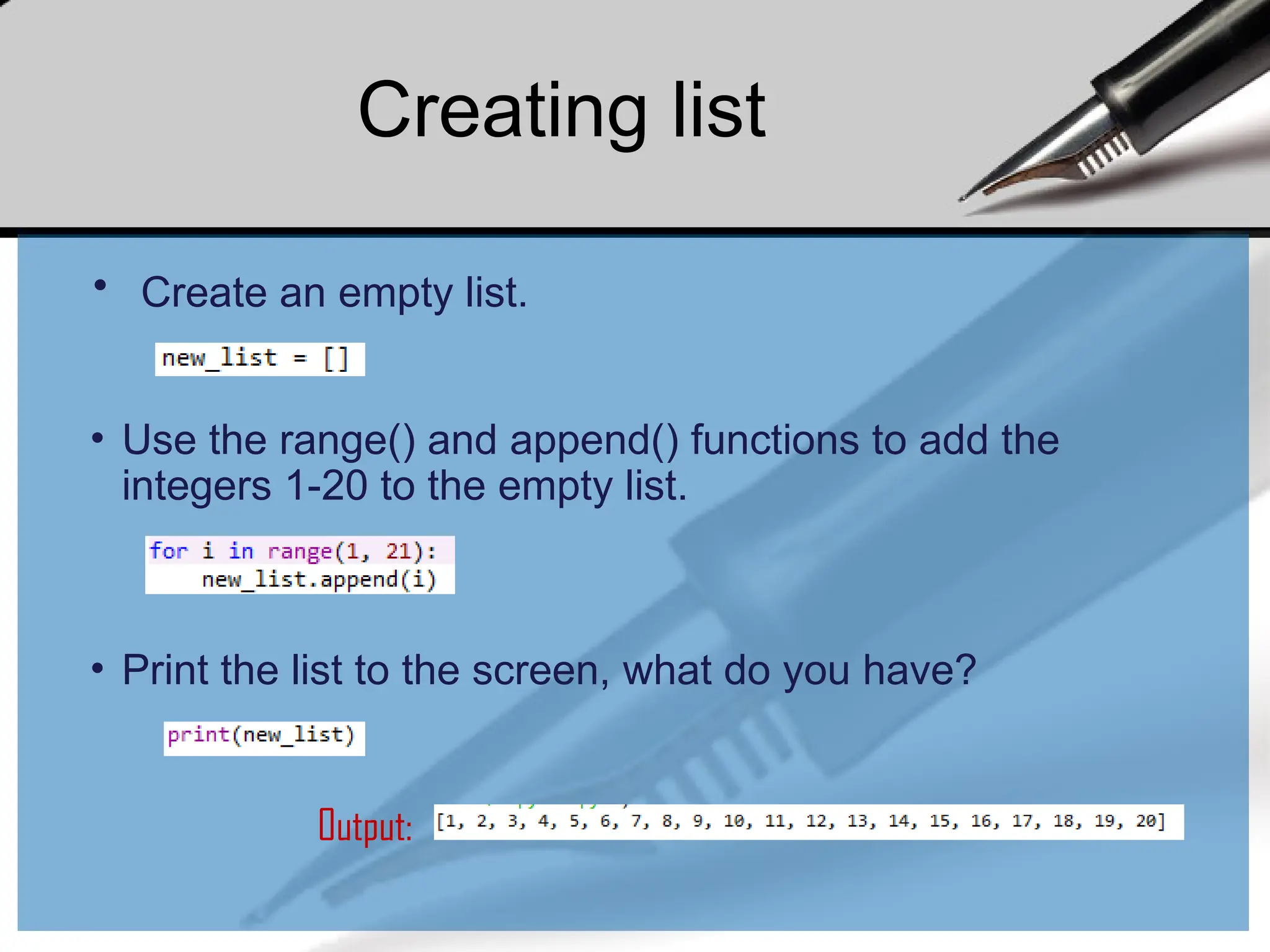
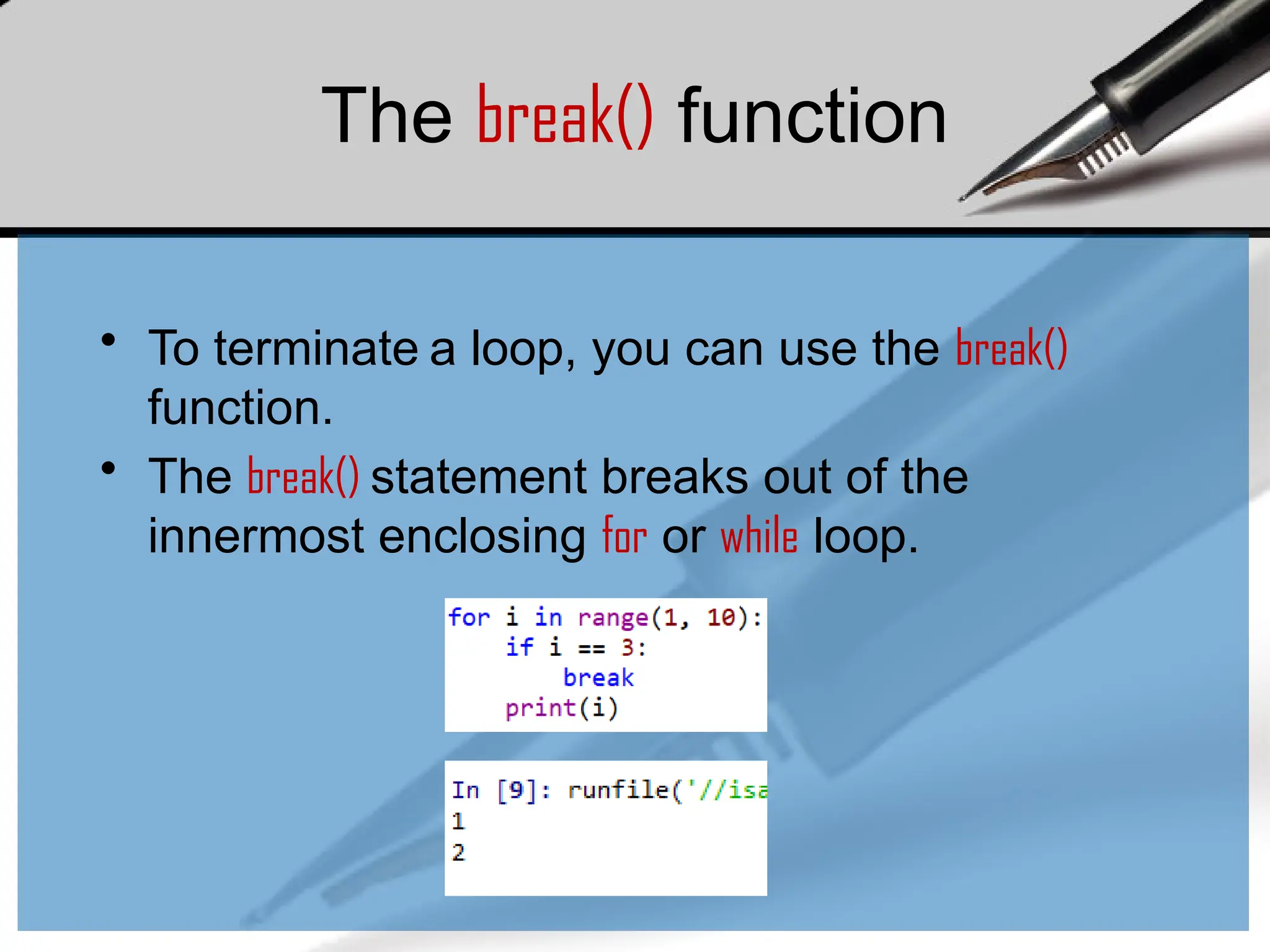
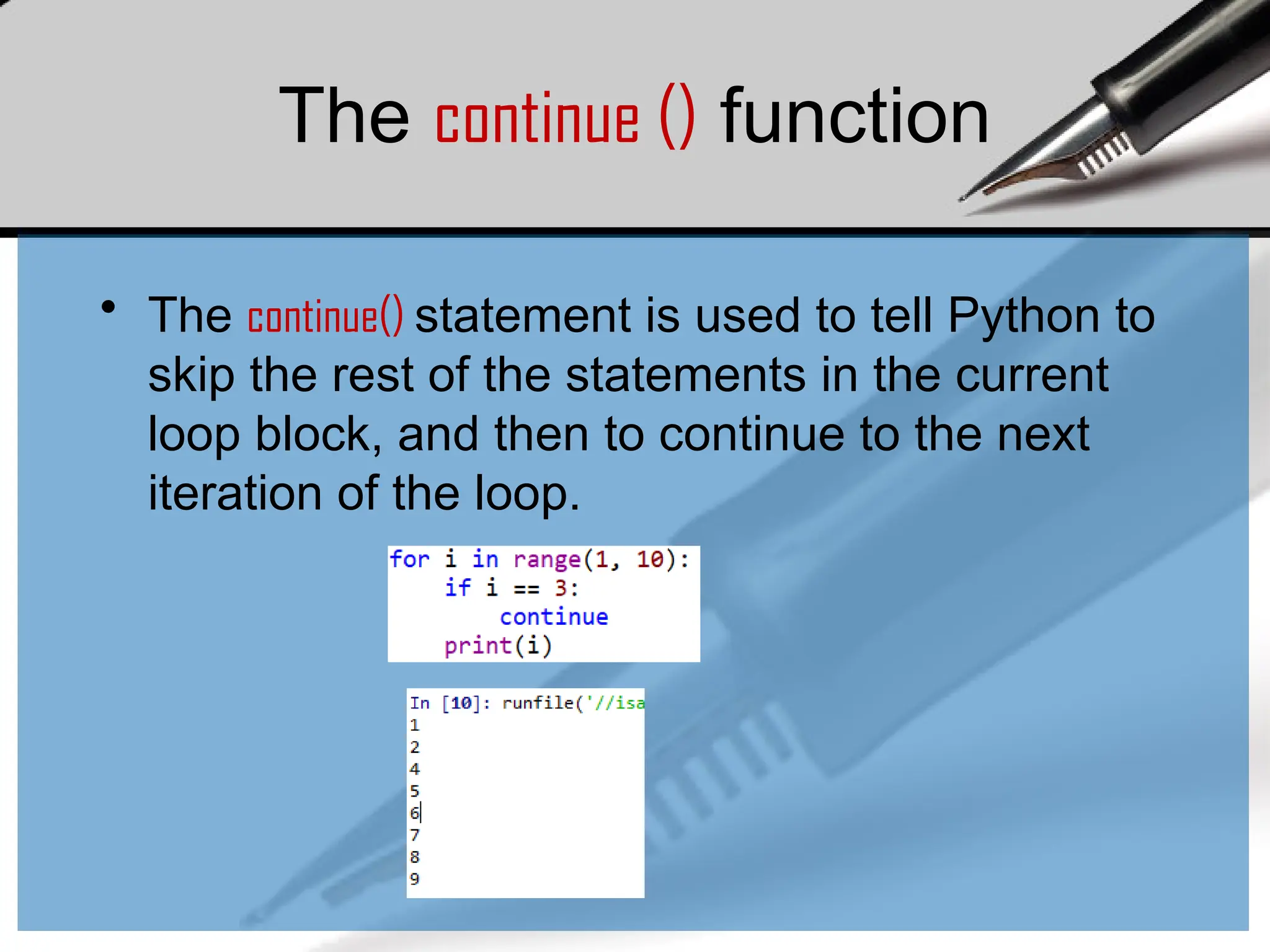
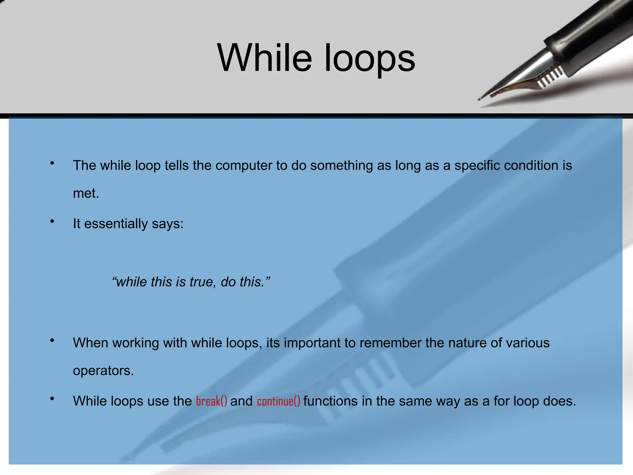
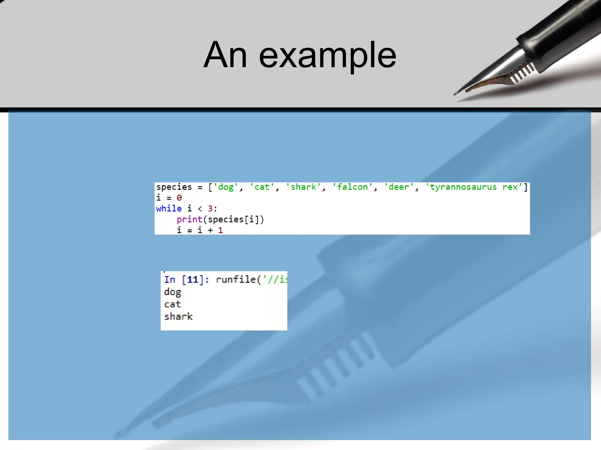
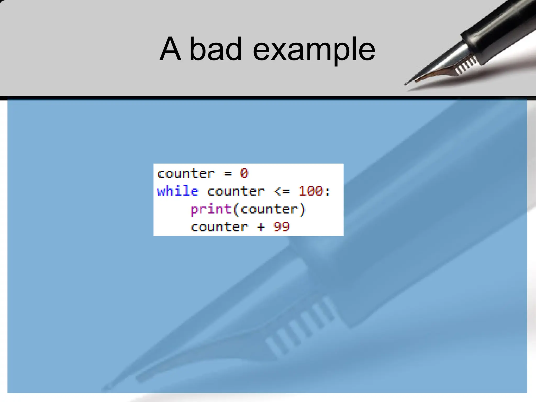
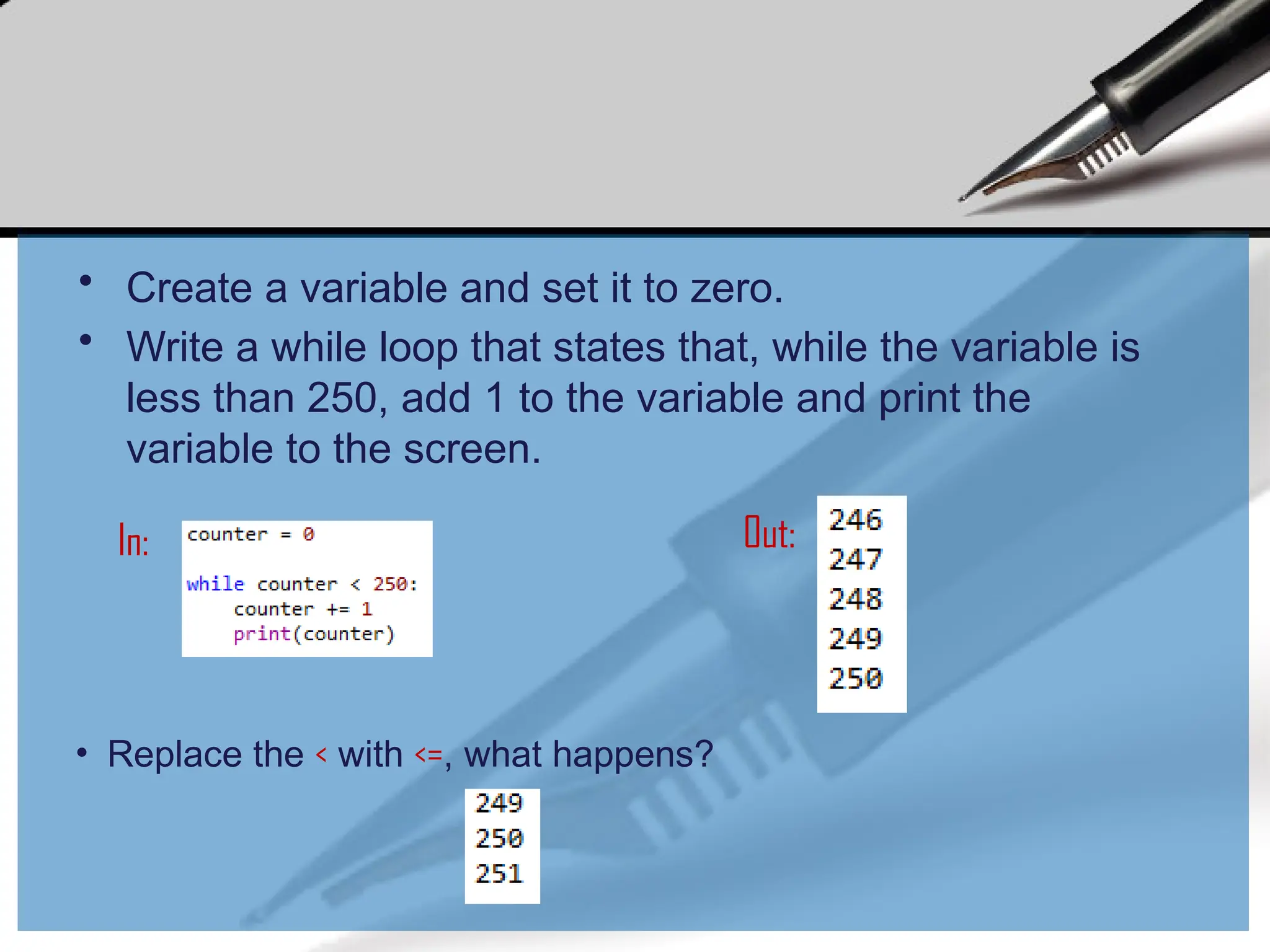
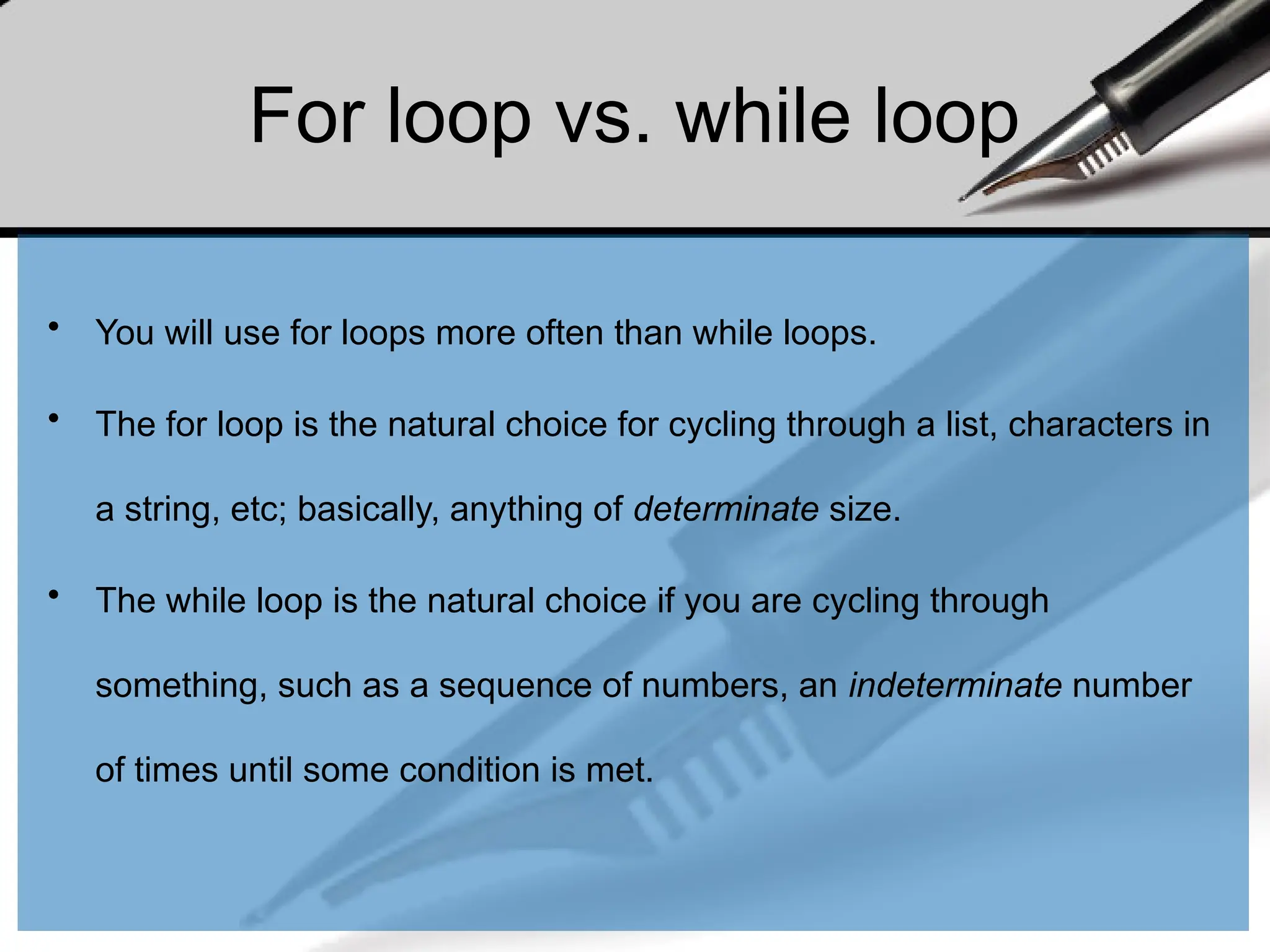
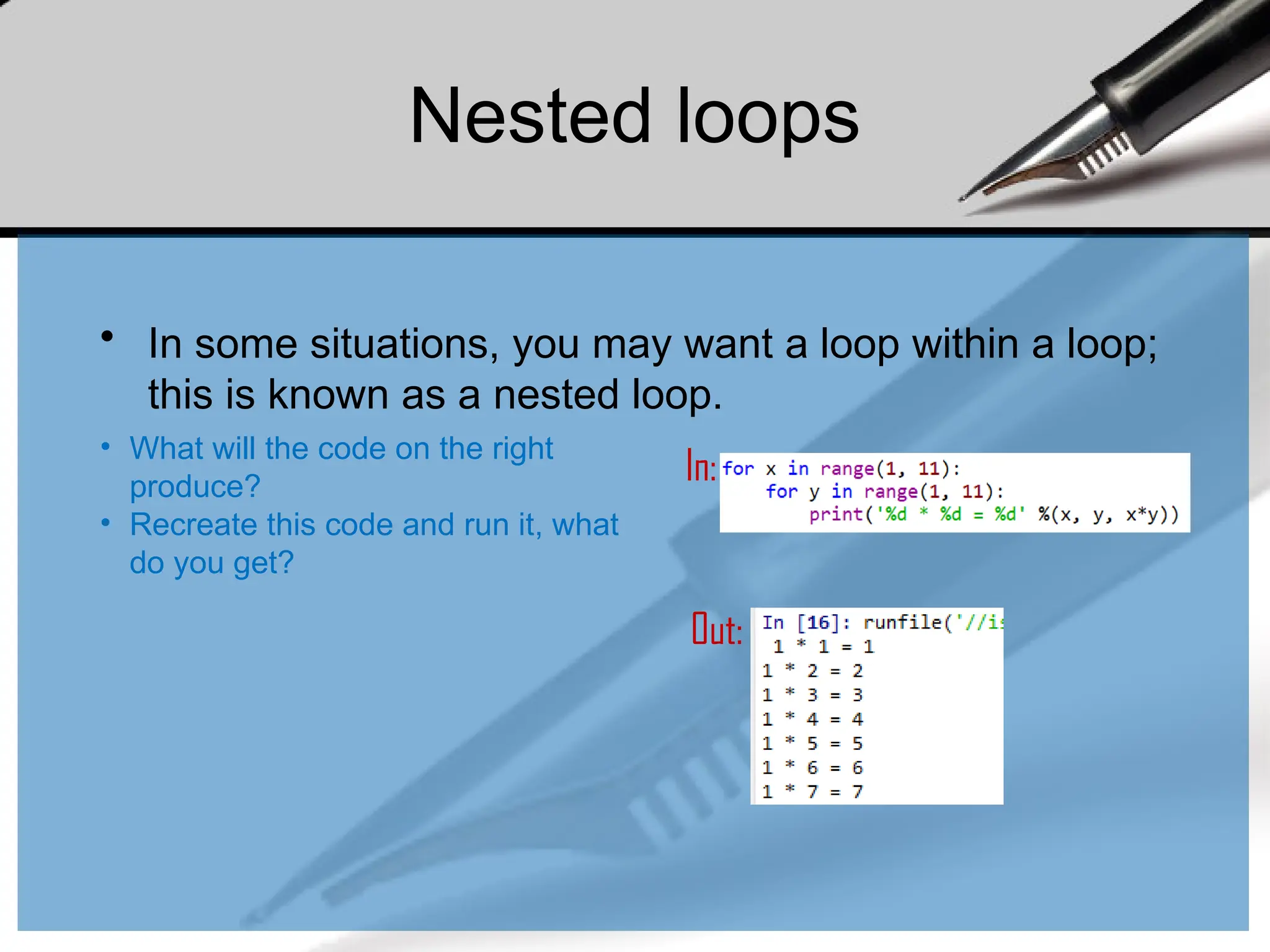
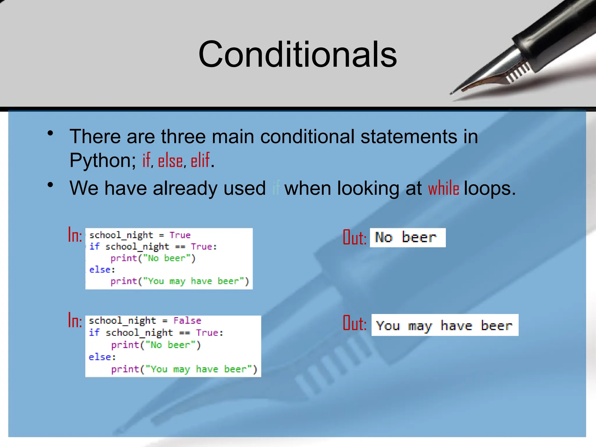

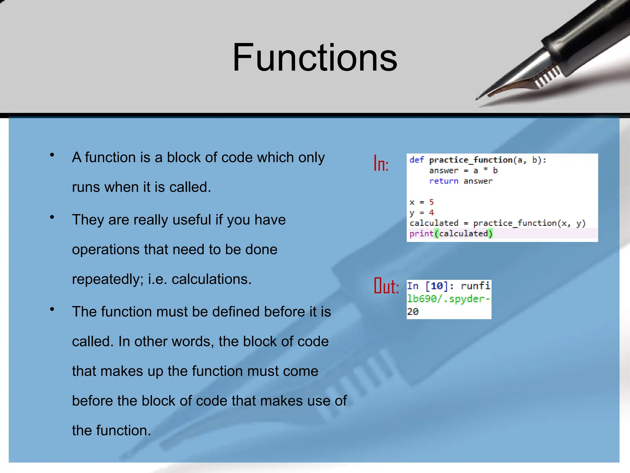
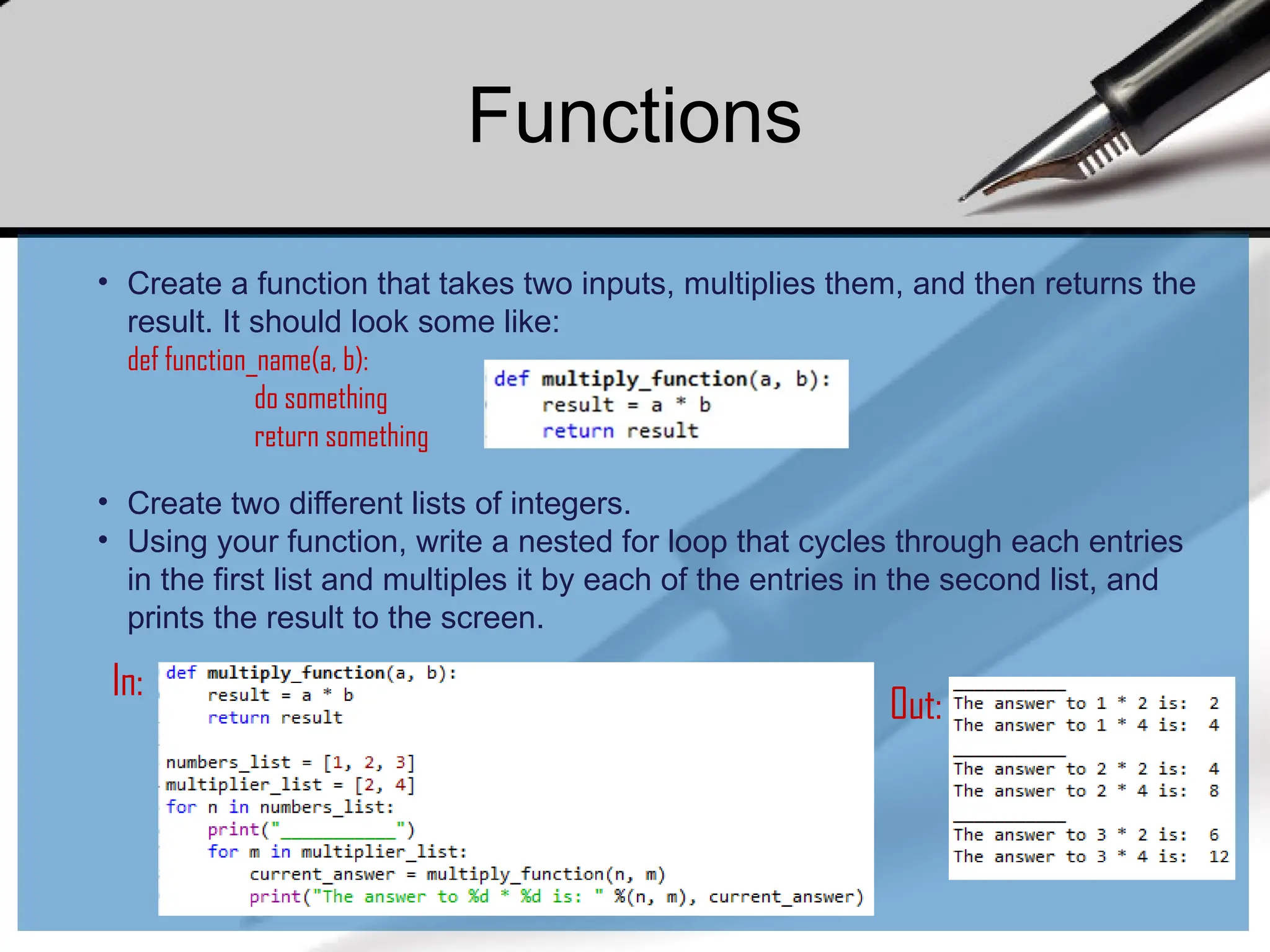
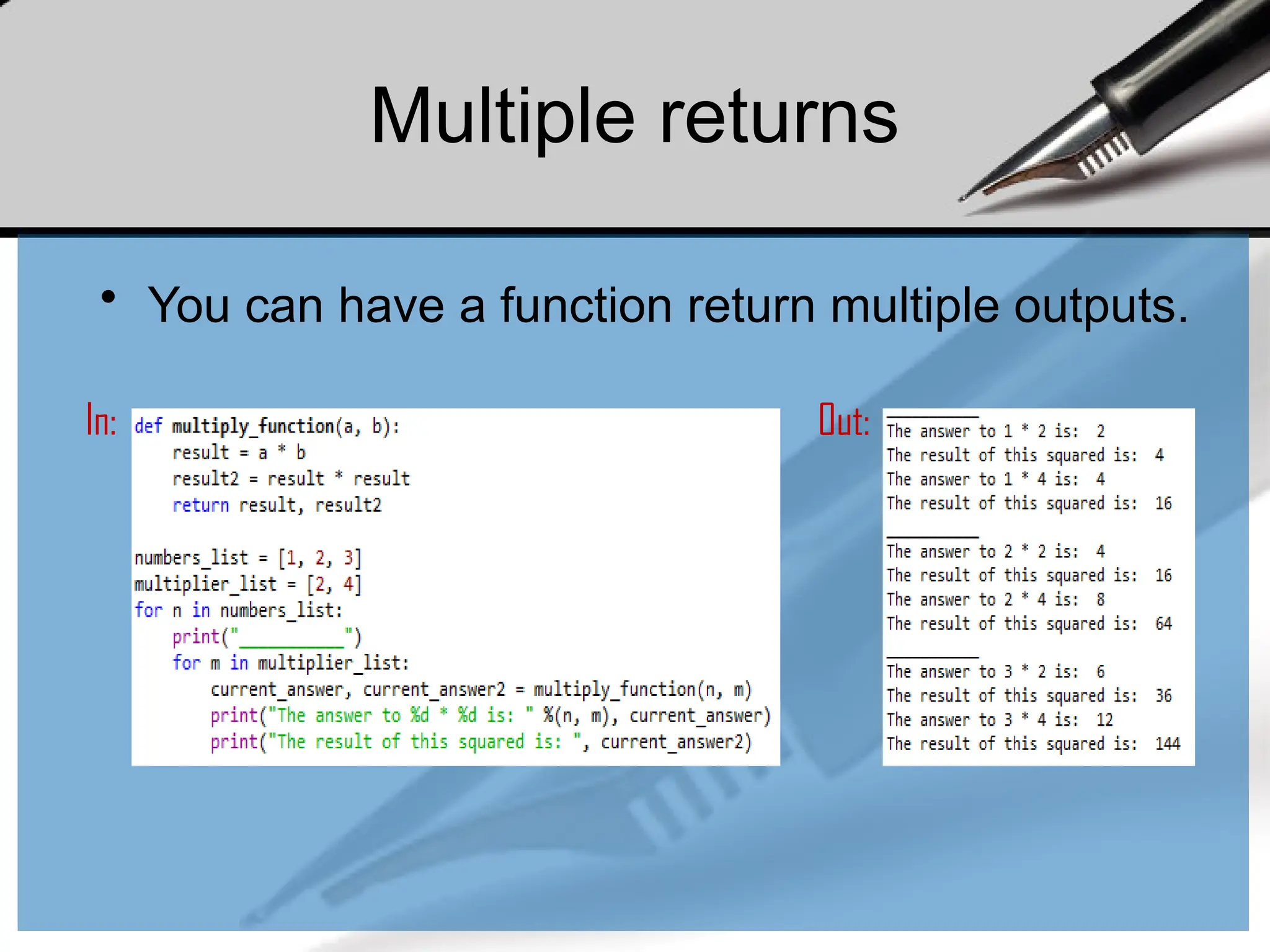
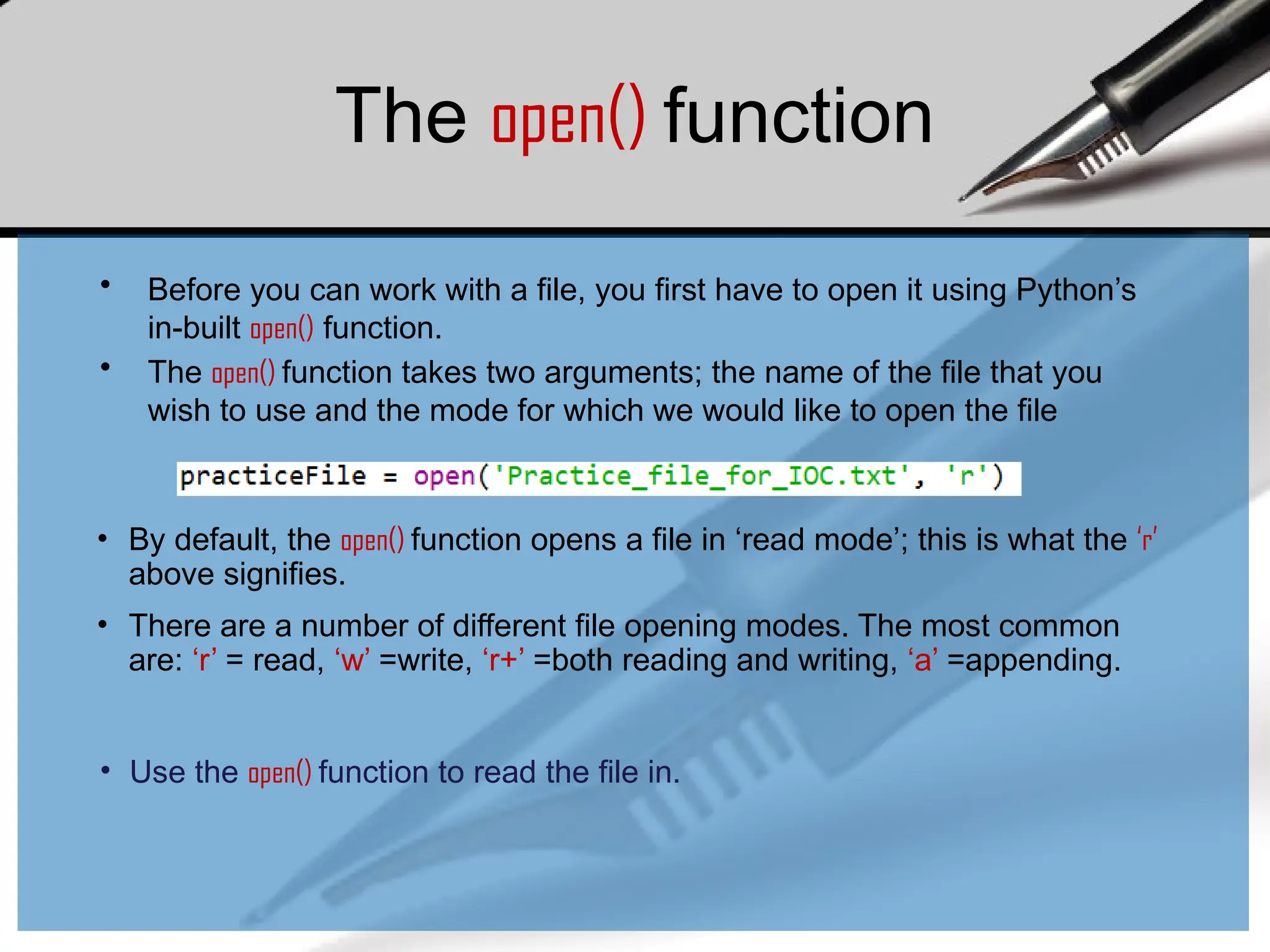

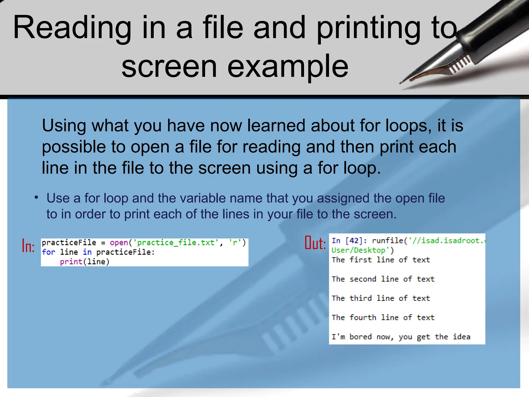
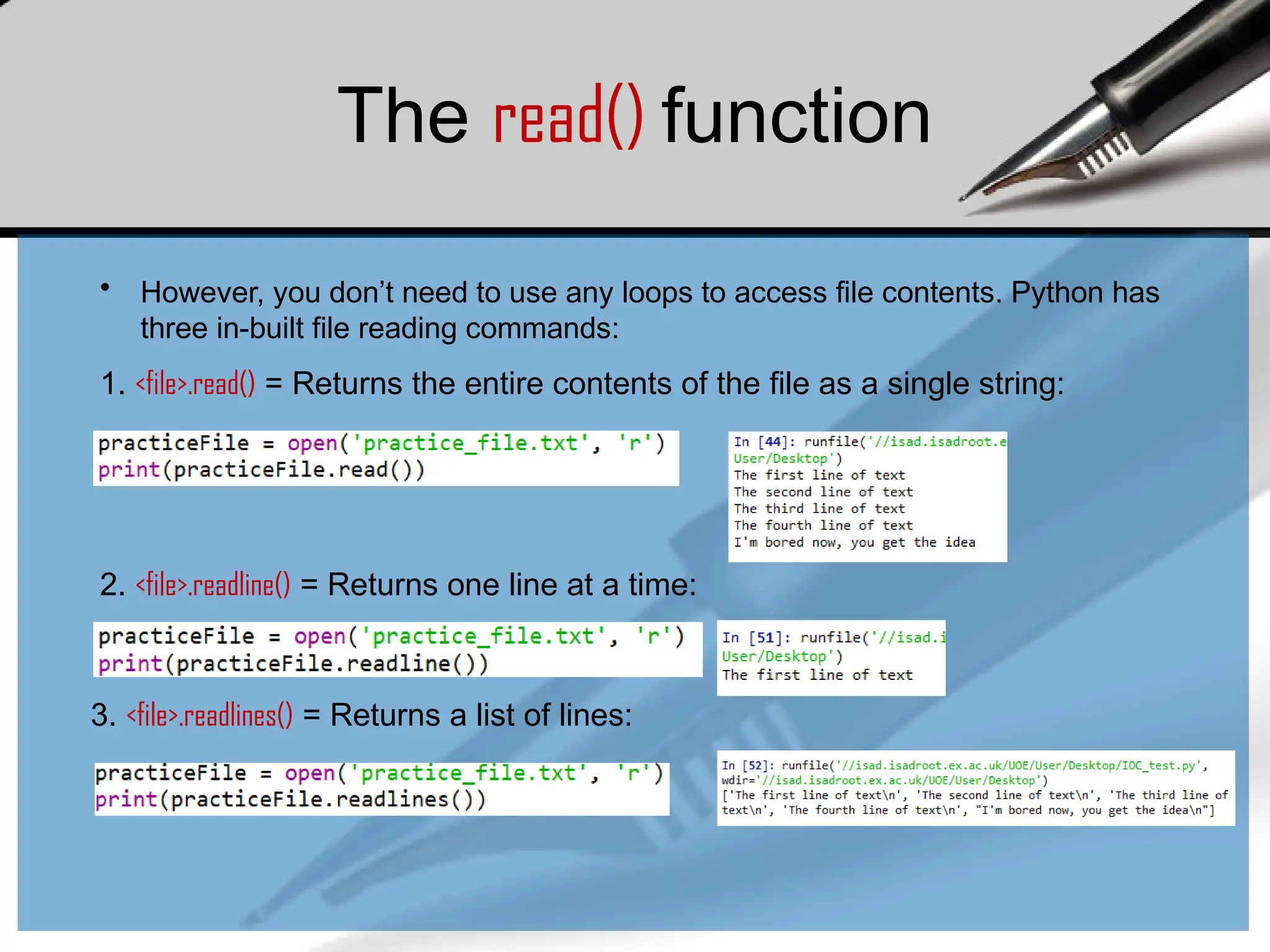
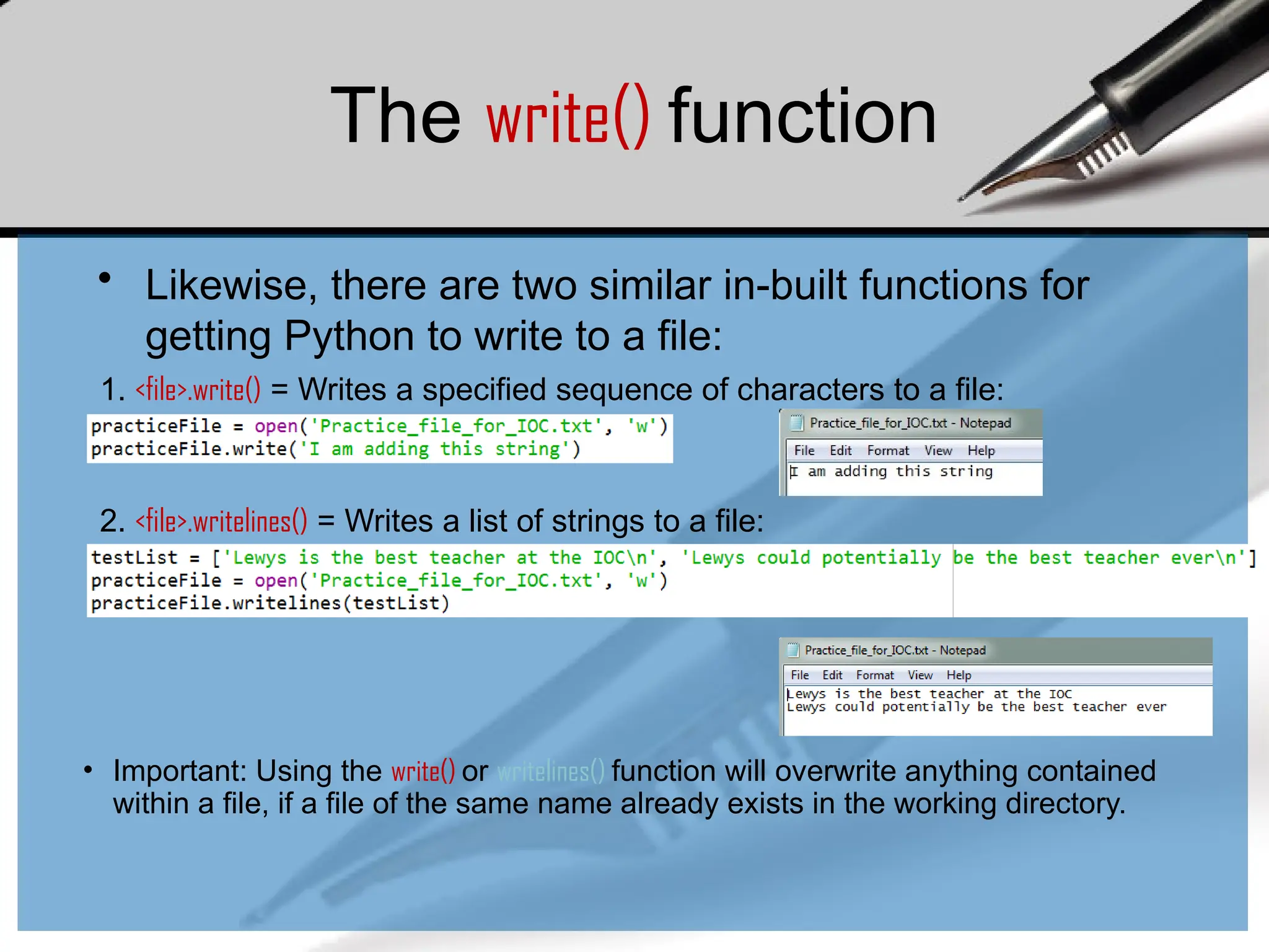

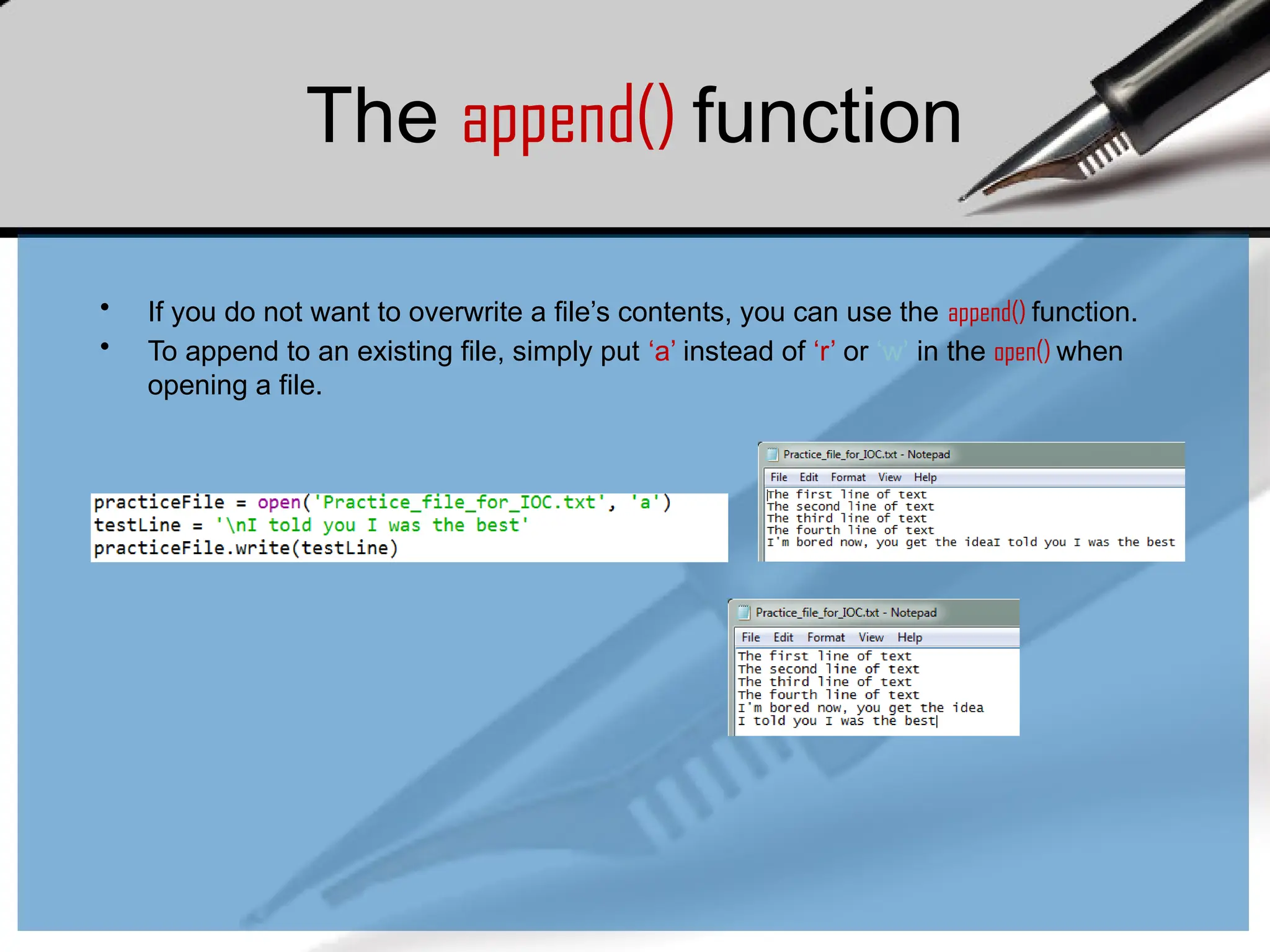

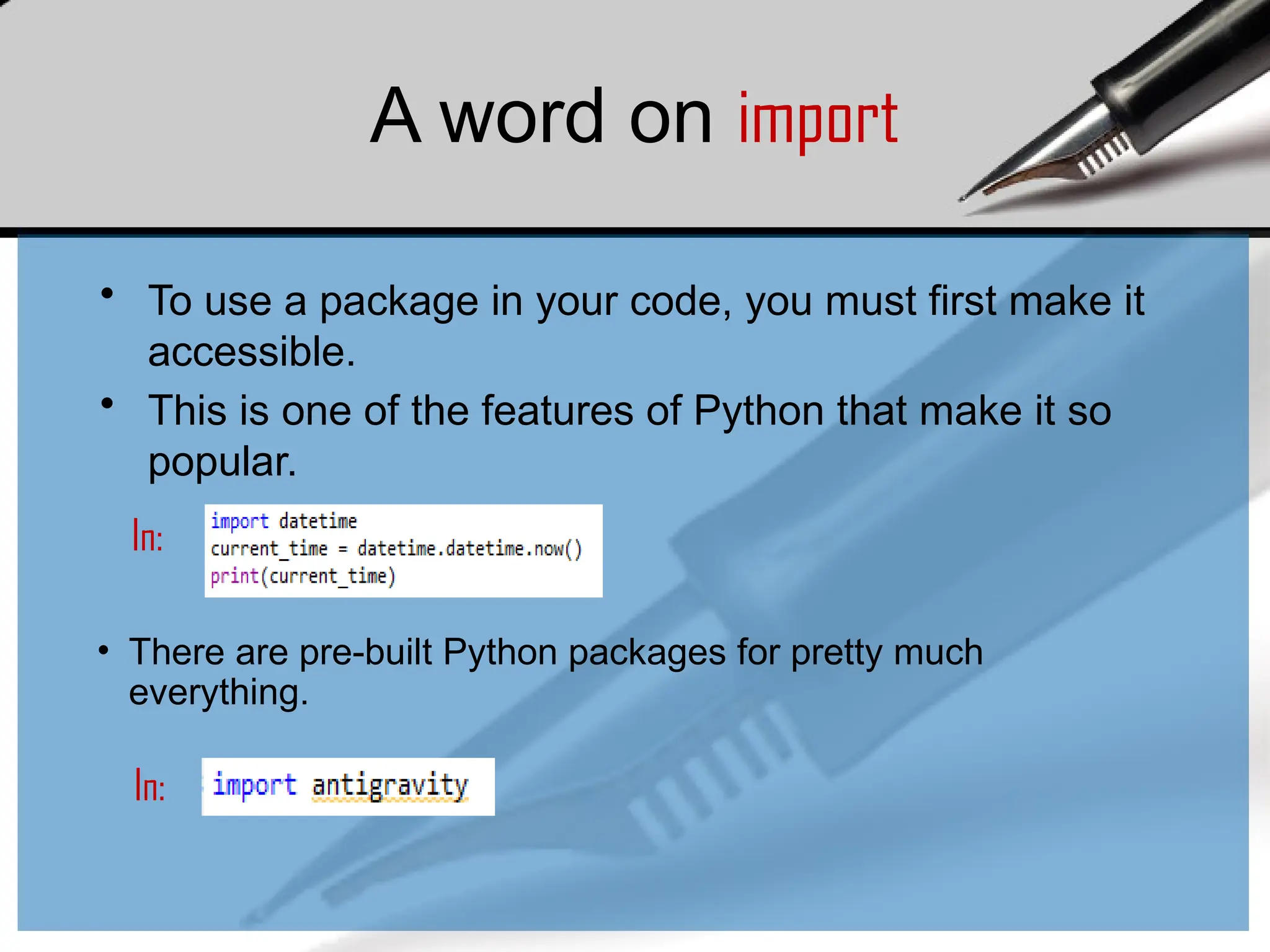
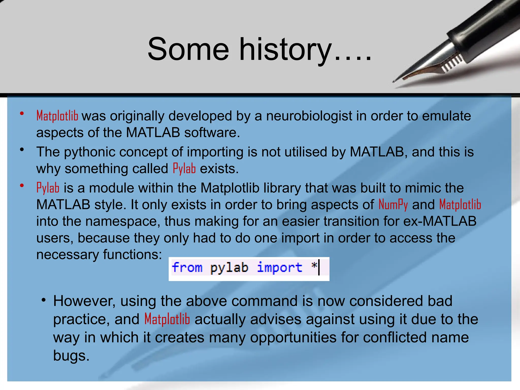
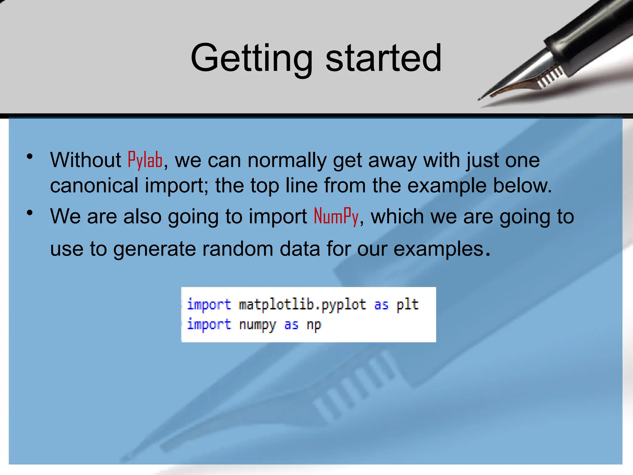
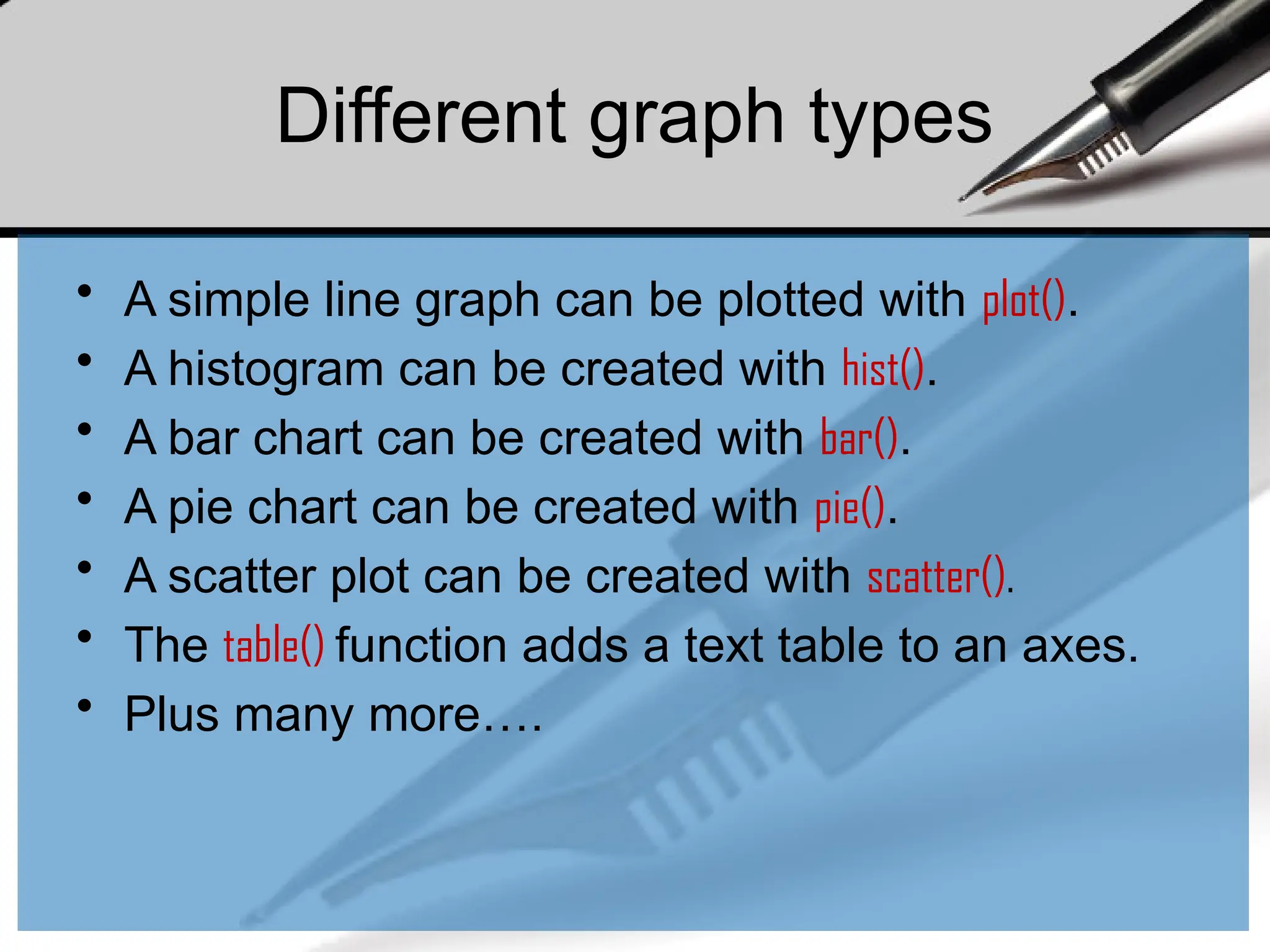
![Our first plot
• You may be wondering why the x-axis ranges
from 0-3 and the y-axis from 1-4.
• If you provide a single list or array to the plot()
command, Matplotlib assumes it is a
sequence of y values, and automatically
generates the x values for you.
• Since python ranges start with 0, the default
x vector has the same length as y but starts
with 0.
• Hence the x data are [0,1,2,3].](https://image.slidesharecdn.com/dalecture1introduction-250915234621-3db310b6/75/DATA-ANALYSIS_Lecture-1-Introduction-pptx-96-2048.jpg)
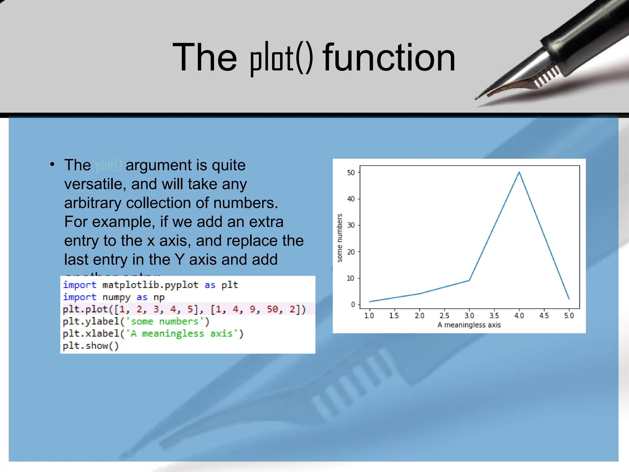
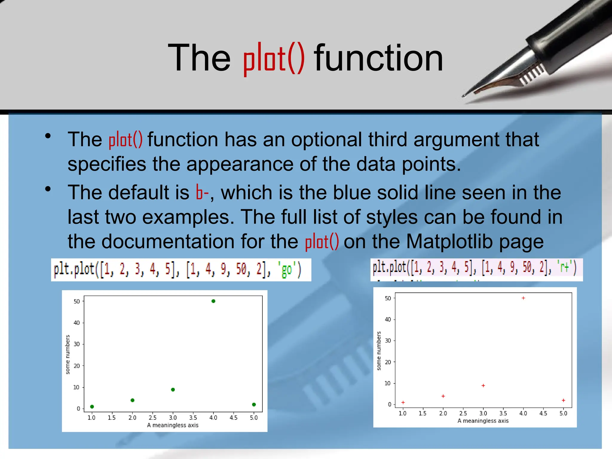
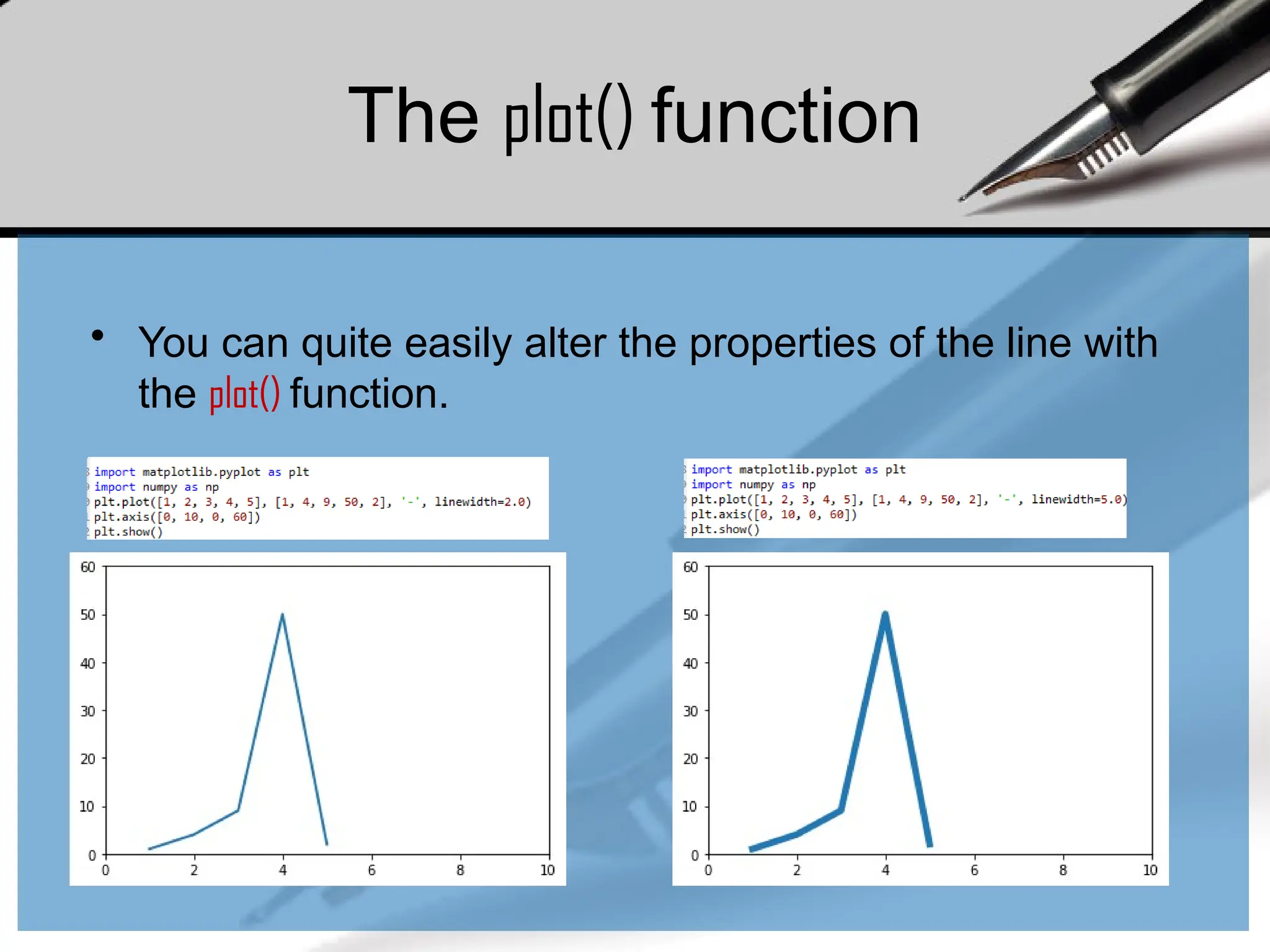
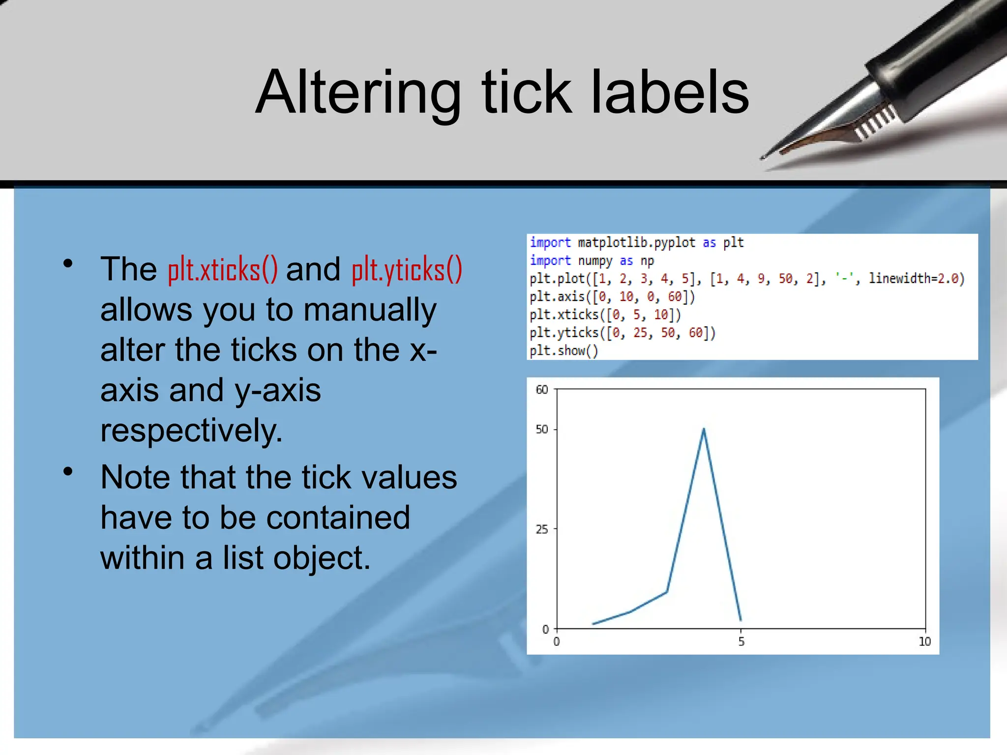
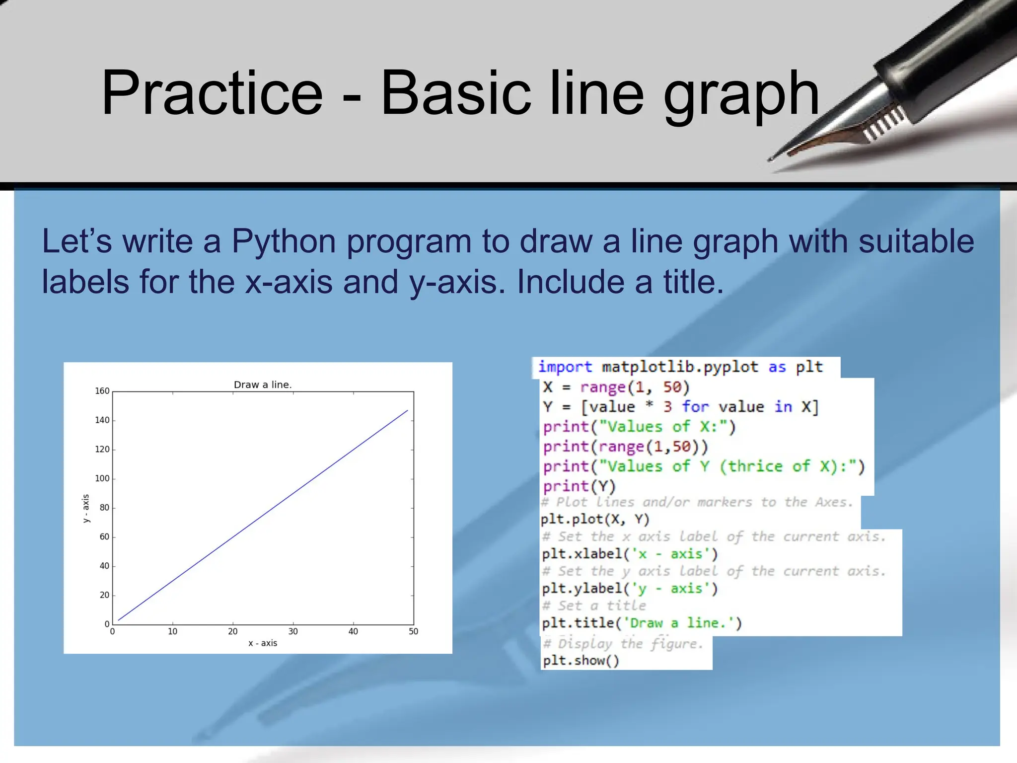
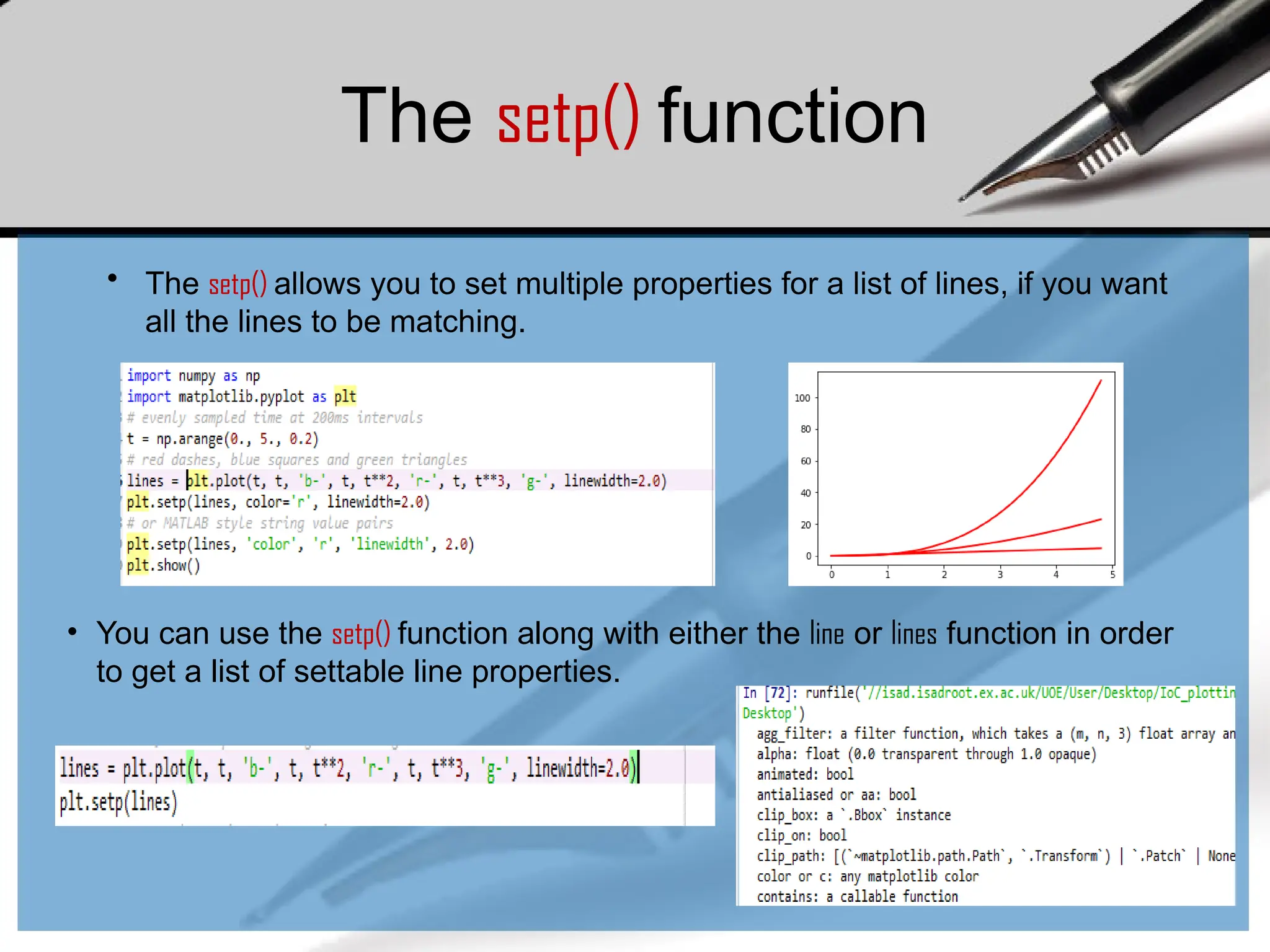
![The axis() function
• The axis() function allows us to specify the range of the axis.
• It requires a list that contains the following:
[The min x-axis value, the max x-axis value, the min y-axis, the max y-axis value]](https://image.slidesharecdn.com/dalecture1introduction-250915234621-3db310b6/75/DATA-ANALYSIS_Lecture-1-Introduction-pptx-103-2048.jpg)
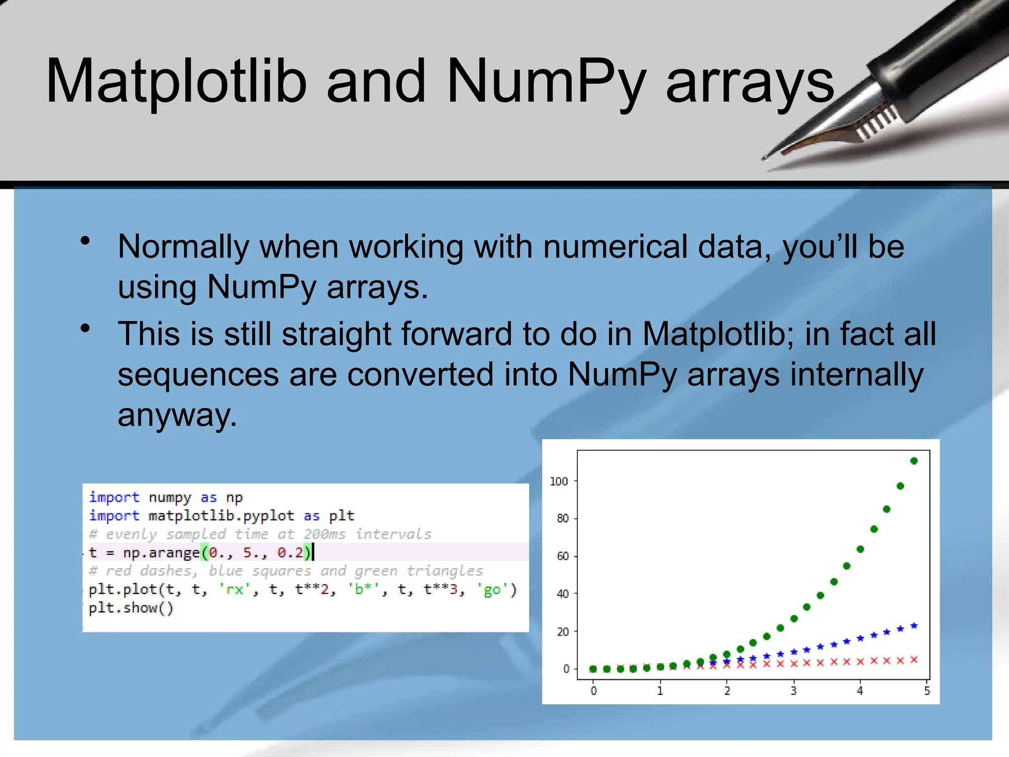
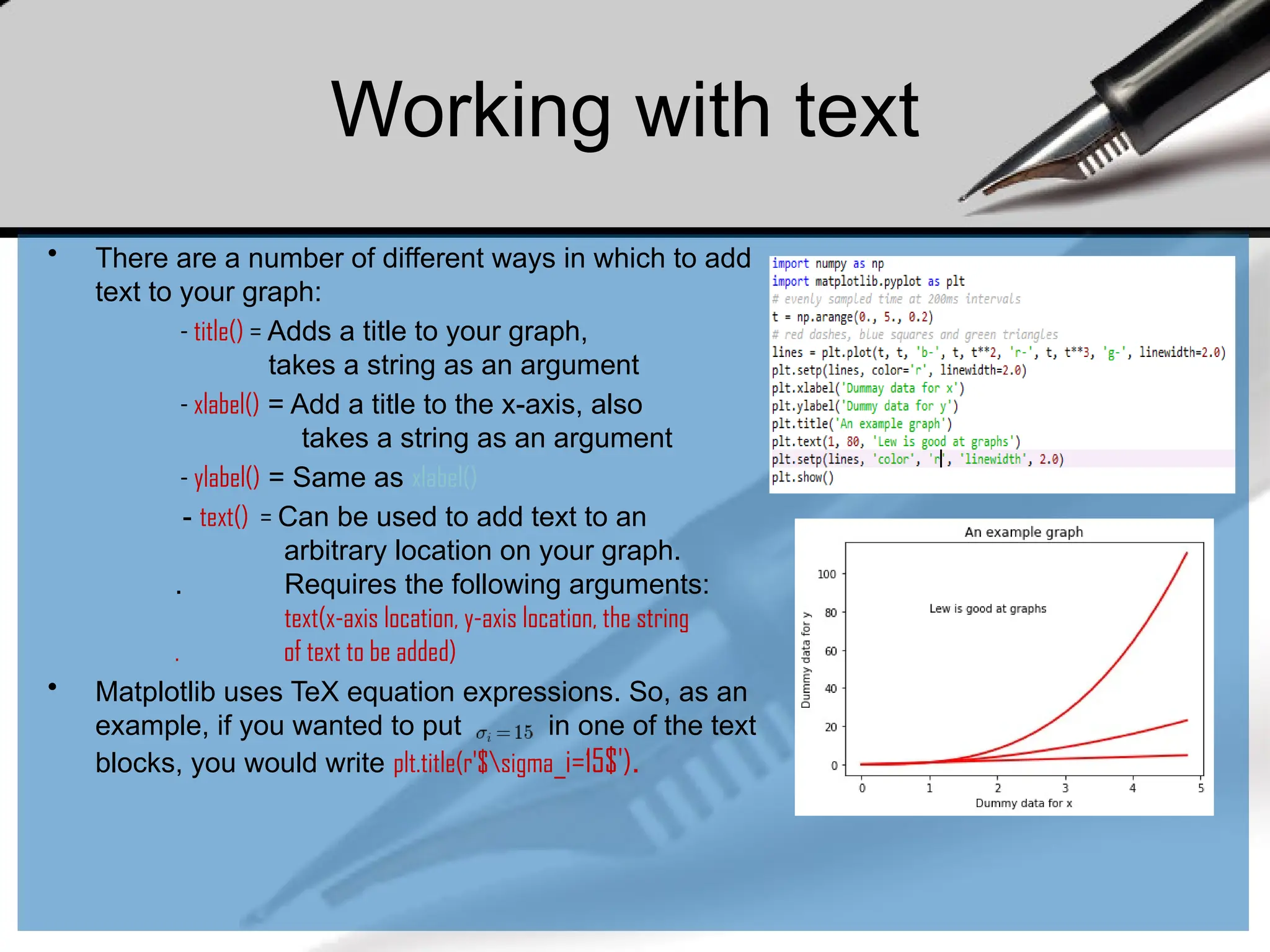
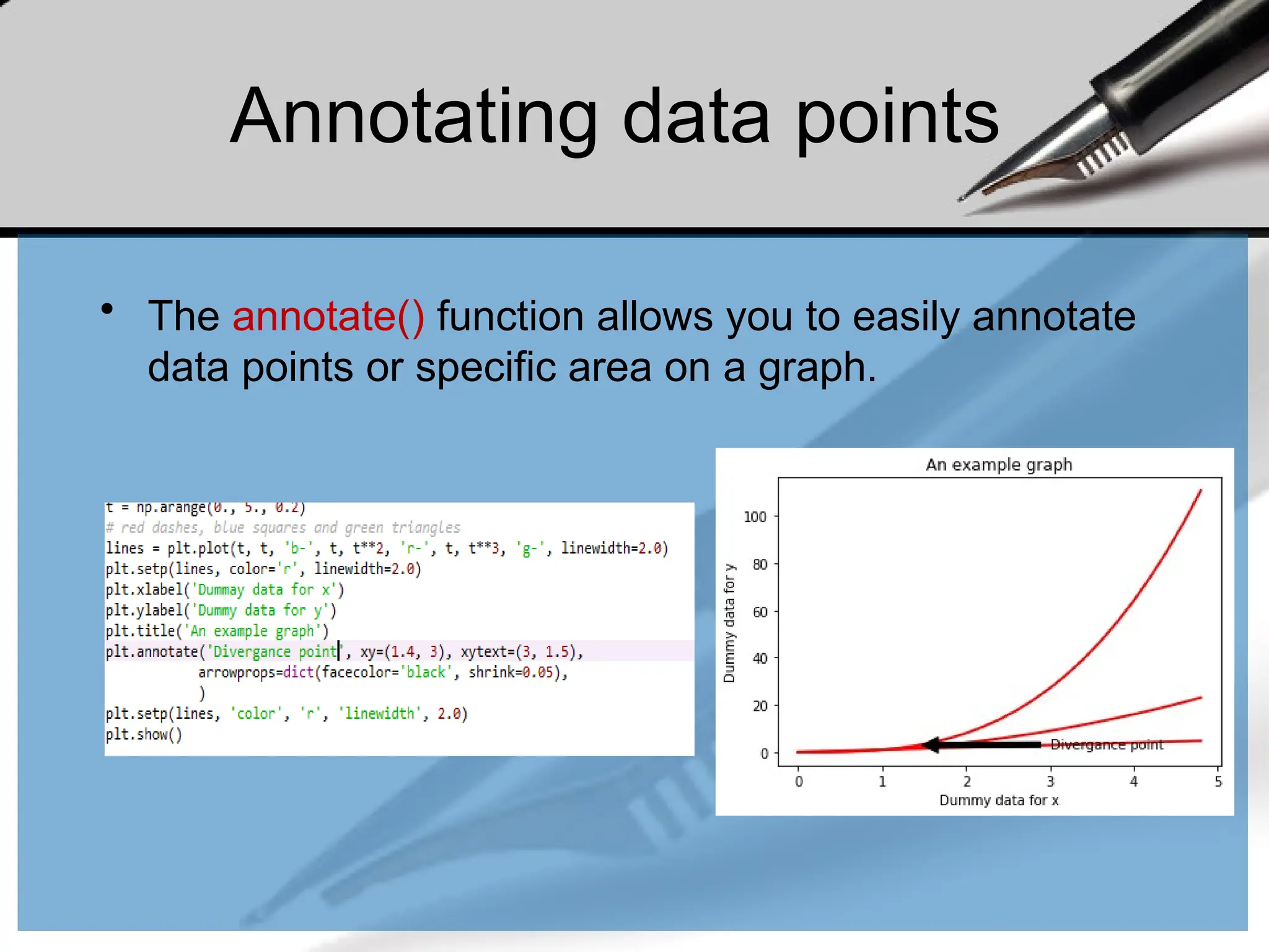
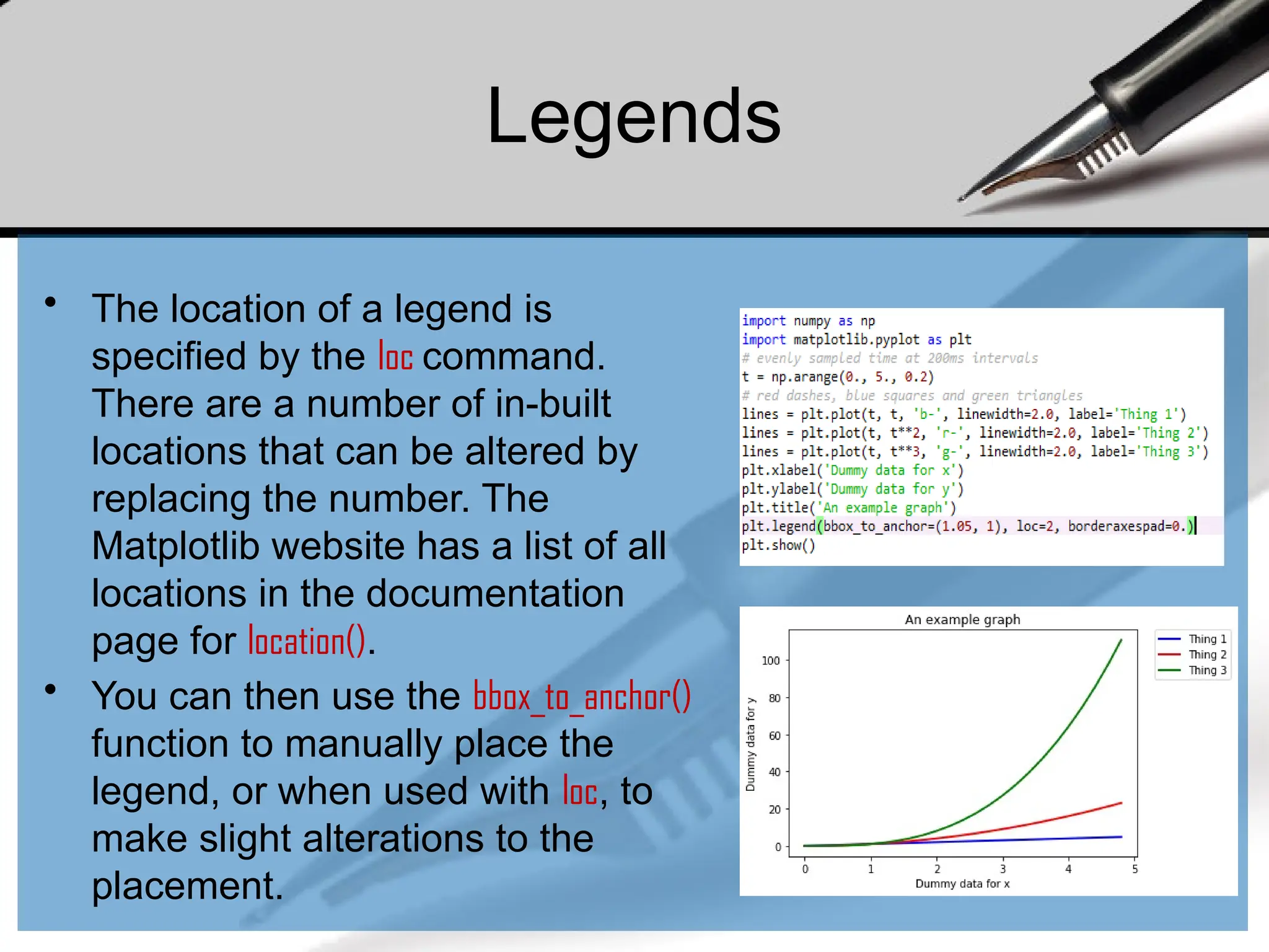
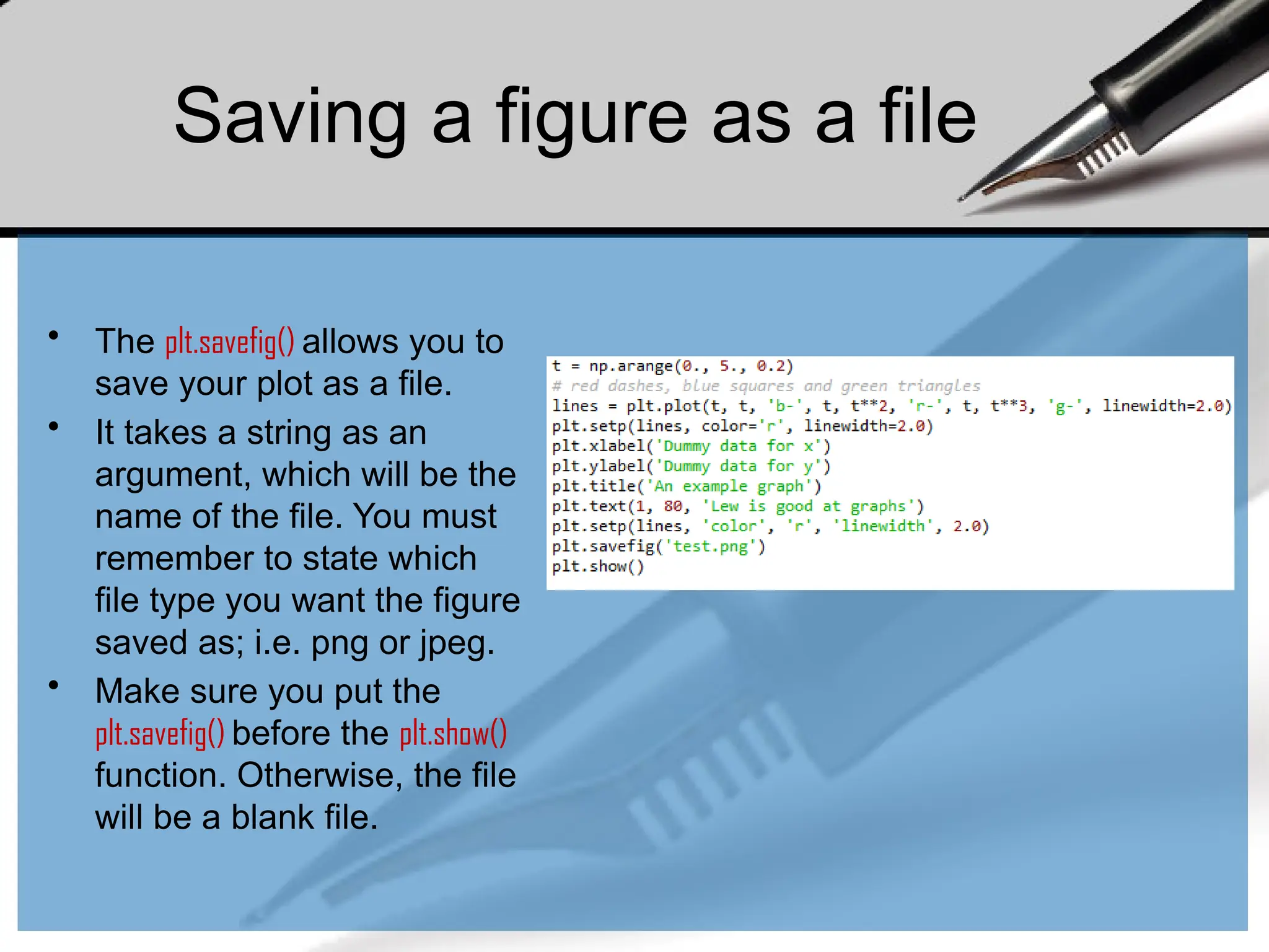
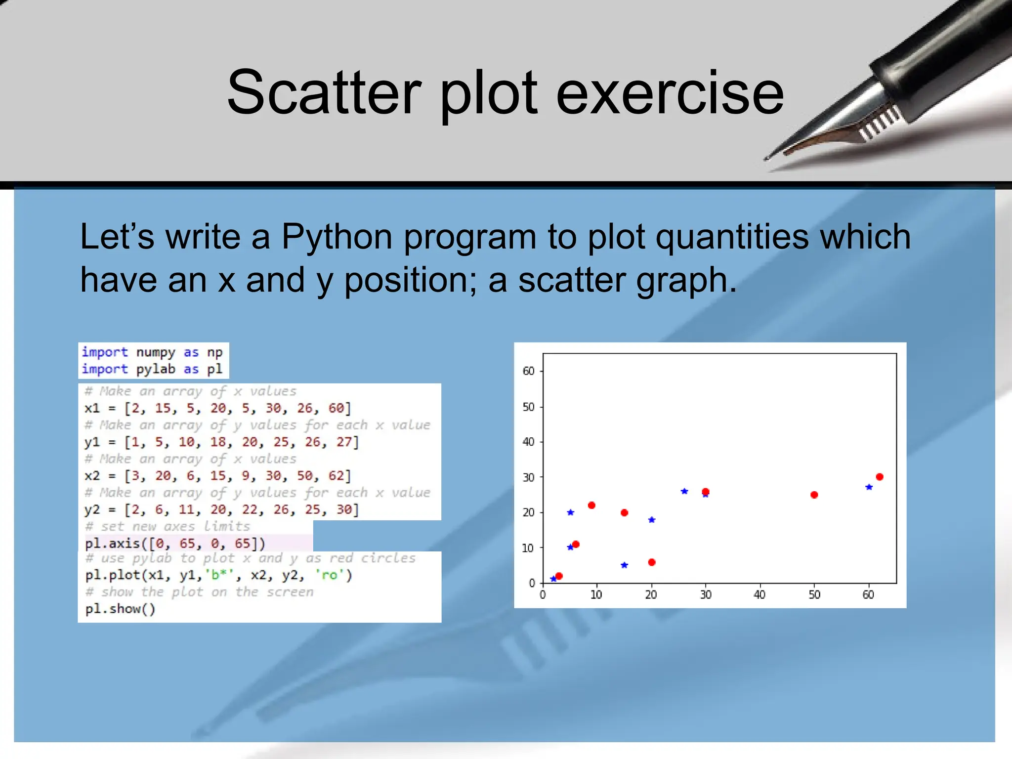

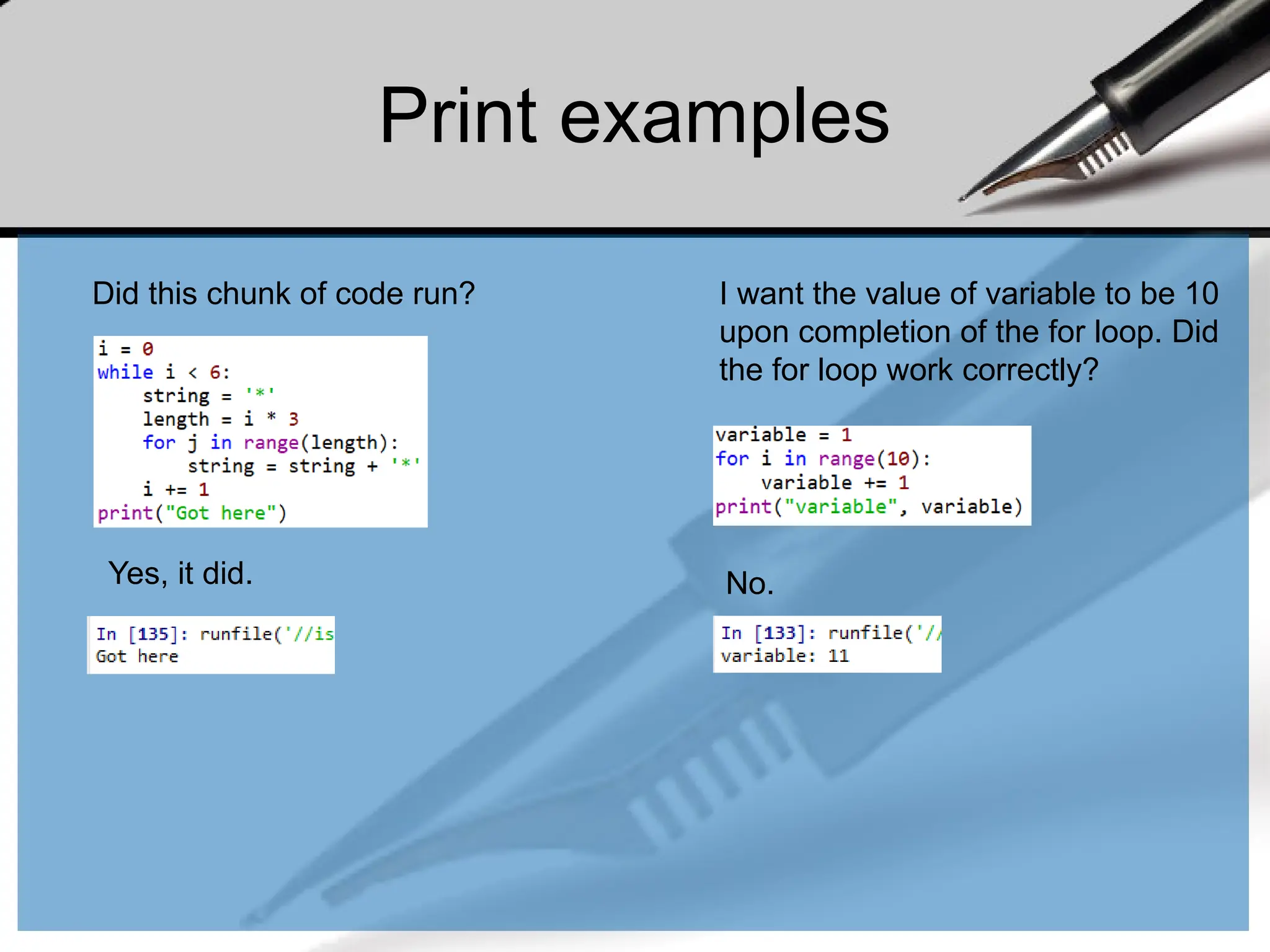
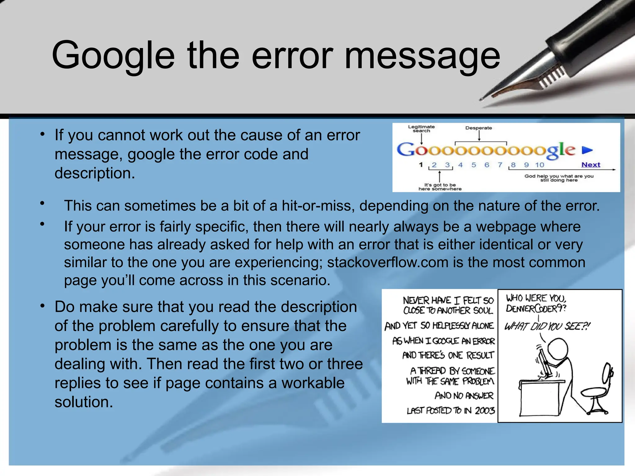


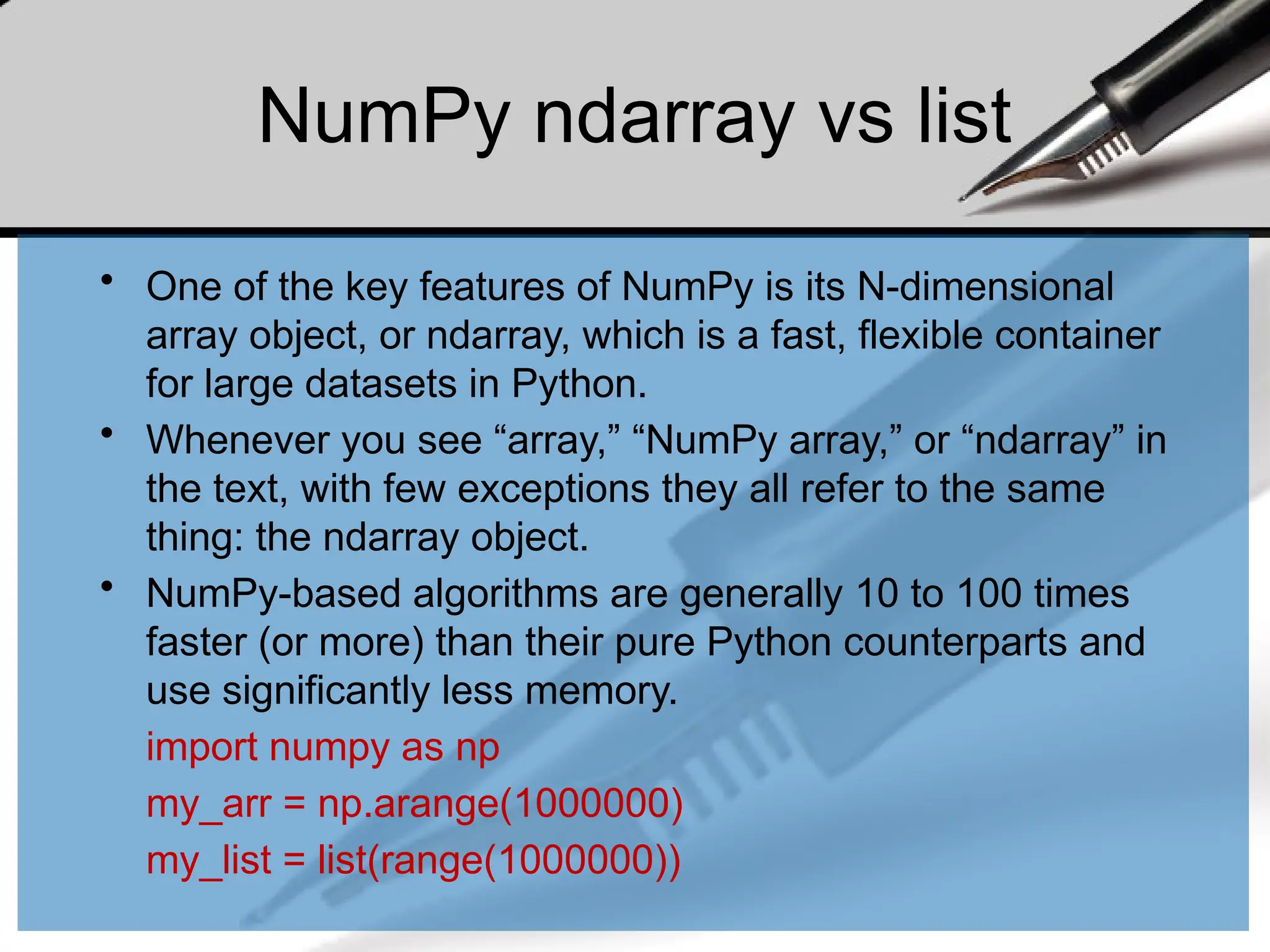
![ndarray
• ndarray is used for storage of homogeneous data
– i.e., all elements the same type
• Every array must have a shape and a dtype
• Supports convenient slicing, indexing and efficient
vectorized computation
import numpy as np
data1 = [6, 7.5, 8, 0, 1]
arr1 = np.array(data1)
print(arr1)
print(arr1.dtype)
print(arr1.shape)
print(arr1.ndim)
[6. 7.5 8. 0. 1. ]
float64
(5,)
1](https://image.slidesharecdn.com/dalecture1introduction-250915234621-3db310b6/75/DATA-ANALYSIS_Lecture-1-Introduction-pptx-126-2048.jpg)
![Creating ndarrays
Using list of lists
import numpy as np
data2 = [[1, 2, 3, 4], [5, 6, 7, 8]] #list of lists
arr2 = np.array(data2)
print(arr2.ndim) #2
print(arr2.shape) # (2,4)](https://image.slidesharecdn.com/dalecture1introduction-250915234621-3db310b6/75/DATA-ANALYSIS_Lecture-1-Introduction-pptx-127-2048.jpg)
![array = np.array([[0,1,2],[2,3,4]])
[[0 1 2]
[2 3 4]]
array = np.zeros((2,3))
[[0. 0. 0.]
[0. 0. 0.]]
array = np.ones((2,3))
[[1. 1. 1.]
[1. 1. 1.]]
array = np.eye(3)
[[1. 0. 0.]
[0. 1. 0.]
[0. 0. 1.]]
array = np.arange(0, 10, 2)
[0, 2, 4, 6, 8]
array = np.random.randint(0,
10, (3,3))
[[6 4 3]
[1 5 6]
[9 8 5]]
Creating ndarrays
arange is an array-valued version of the built-in Python range function](https://image.slidesharecdn.com/dalecture1introduction-250915234621-3db310b6/75/DATA-ANALYSIS_Lecture-1-Introduction-pptx-128-2048.jpg)
![Arithmatic with NumPy Arrays
• Any arithmetic operations between equal-size
arrays applies the operation element-wise:
arr = np.array([[1., 2., 3.], [4., 5., 6.]])
print(arr)
[[1. 2. 3.]
[4. 5. 6.]]
print(arr * arr)
[[ 1. 4. 9.]
[16. 25. 36.]]
print(arr - arr)
[[0. 0. 0.]
[0. 0. 0.]]](https://image.slidesharecdn.com/dalecture1introduction-250915234621-3db310b6/75/DATA-ANALYSIS_Lecture-1-Introduction-pptx-129-2048.jpg)
![Arithmatic with NumPy Arrays
• Arithmetic operations with scalars propagate the scalar argument to
each element in the array:
• Comparisons between arrays of the same size yield boolean arrays:
arr = np.array([[1., 2., 3.], [4., 5., 6.]])
print(arr)
[[1. 2. 3.]
[4. 5. 6.]]
print(arr **2)
[[ 1. 4. 9.]
[16. 25. 36.]]
arr2 = np.array([[0., 4., 1.], [7., 2., 12.]])
print(arr2)
[[ 0. 4. 1.]
[ 7. 2. 12.]]
print(arr2 > arr)
[[False True False]
[ True False True]]](https://image.slidesharecdn.com/dalecture1introduction-250915234621-3db310b6/75/DATA-ANALYSIS_Lecture-1-Introduction-pptx-130-2048.jpg)
![Indexing and Slicing
• One-dimensional arrays are simple; on the
surface they act similarly to Python lists:
arr = np.arange(10)
print(arr) # [0 1 2 3 4 5 6 7 8 9]
print(arr[5]) #5
print(arr[5:8]) #[5 6 7]
arr[5:8] = 12
print(arr) #[ 0 1 2 3 4 12 12 12 8 9]](https://image.slidesharecdn.com/dalecture1introduction-250915234621-3db310b6/75/DATA-ANALYSIS_Lecture-1-Introduction-pptx-131-2048.jpg)
![Indexing and Slicing
• As you can see, if you assign a scalar value to a slice, as in arr[5:8] =
12, the value is propagated (or broadcasted) to the entire selection.
• An important first distinction from Python’s built-in lists is that array
slices are views on the original array.
– This means that the data is not copied, and any modifications to the view
will be reflected in the source array.
arr = np.arange(10)
print(arr) # [0 1 2 3 4 5 6 7 8 9]
arr_slice = arr[5:8]
print(arr_slice) # [5 6 7]
arr_slice[1] = 12345
print(arr) # [ 0 1 2 3 4 5 12345 7 8 9]
arr_slice[:] = 64
print(arr) # [ 0 1 2 3 4 64 64 64 8 9]](https://image.slidesharecdn.com/dalecture1introduction-250915234621-3db310b6/75/DATA-ANALYSIS_Lecture-1-Introduction-pptx-132-2048.jpg)
![Indexing
• In a two-dimensional array, the elements at each index are
no longer scalars but rather one-dimensional arrays:
• Thus, individual elements can be accessed recursively.
But that is a bit too much work, so you can pass a comma-
separated list of indices to select individual elements.
• So these are equivalent:
arr2d = np.array([[1, 2, 3], [4, 5, 6], [7, 8, 9]])
print(arr2d[2]) # [7 8 9]
print(arr2d[0][2]) # 3
print(arr2d[0, 2]) #3](https://image.slidesharecdn.com/dalecture1introduction-250915234621-3db310b6/75/DATA-ANALYSIS_Lecture-1-Introduction-pptx-133-2048.jpg)
![Activity
• Consider the two-dimensional array, arr2d.
• Write a code to slice this array to display the last
column,
[[3] [6] [9]]
• Write a code to slice this array to display the last
2 elements of middle array,
[5 6]
arr2d = np.array([[1, 2, 3], [4, 5, 6], [7, 8, 9]])](https://image.slidesharecdn.com/dalecture1introduction-250915234621-3db310b6/75/DATA-ANALYSIS_Lecture-1-Introduction-pptx-134-2048.jpg)
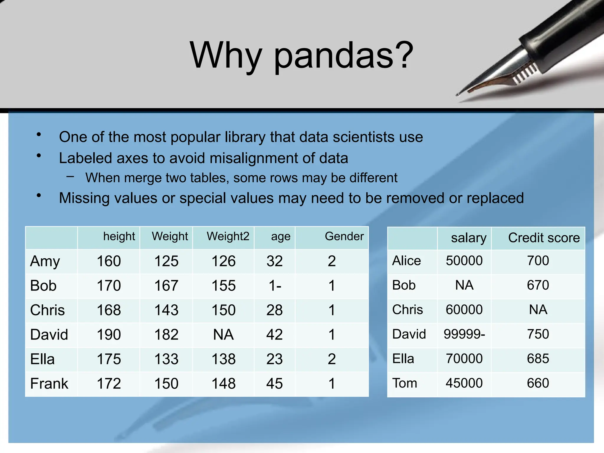
![Series
• One dimensional array-like object
• It contains array of data (of any NumPy data type) with
associated indexes. (Indexes can be strings or integers
or other data types.)
• By default , the series will get indexing from 0 to N where
N = size -1
from pandas import Series, DataFrame
import pandas as pd
obj = Series([4, 7, -5, 3])
print(obj)
print(obj.index)
print(obj.values)
#Output
0 4
1 7
2 -5
3 3
dtype: int64
RangeIndex(start=0, stop=4, step=1)
[ 4 7 -5 3]](https://image.slidesharecdn.com/dalecture1introduction-250915234621-3db310b6/75/DATA-ANALYSIS_Lecture-1-Introduction-pptx-138-2048.jpg)
![Series – referencing elements
obj2 = Series([4, 7, -5, 3], index=['d', 'b', 'a', 'c'])
print(obj2)
#Output
d 4
b 7
a -5
c 3
dtype: int64
print(obj2.index)
#Output
Index(['d', 'b', 'a', 'c'], dtype='object')
print(obj2.values)
#Output
[ 4 7 -5 3]
print(obj2['a'])
#Output
-5
obj2['d']= 10
print(obj2[['d', 'c', 'a']])
#Output
d 10
c 3
a -5
dtype: int64
print(obj2[:2])
#Output
d 10
b 7
dtype: int64
print(obj2.a)
#Output
-5](https://image.slidesharecdn.com/dalecture1introduction-250915234621-3db310b6/75/DATA-ANALYSIS_Lecture-1-Introduction-pptx-139-2048.jpg)
![Series – array/dict operations
numpy array operations can also be applied,
which will preserve the index-value link
obj4 = obj3[obj3>0]
print(obj4)
#output
d 10
b 7
c 3
dtype: int64
print(obj3**2)
#output
d 100
b 49
a 25
c 9
dtype: int64
print(‘b’ in obj3)
#output
true
Can be thought of as a dict.
Can be constructed from a dict directly.
obj3 = Series({'d': 4, 'b': 7, 'a': -5, 'c':3 })
print(obj3)
#output
d 4
b 7
a -5
c 3
dtype: int64](https://image.slidesharecdn.com/dalecture1introduction-250915234621-3db310b6/75/DATA-ANALYSIS_Lecture-1-Introduction-pptx-140-2048.jpg)
![Series – from dictionary
sdata = {'Texas': 10, 'Ohio': 20, 'Oregon': 15, 'Utah': 18}
states = ['Texas', 'Ohio', 'Oregon', 'Iowa']
obj4 = Series(sdata, index=states)
print(obj4)
#output
Texas 10.0
Ohio 20.0
Oregon 15.0
Iowa NaN
dtype: float64
Missing value
print(pd.isnull(obj4))
#output
Texas False
Ohio False
Oregon False
Iowa True
dtype: bool
print(pd.notnull(obj4))
#output
Texas True
Ohio True
Oregon True
Iowa False
dtype: bool
print(obj4[obj4.notnull()])
#output
Texas 10.0
Ohio 20.0
Oregon 15.0
dtype: float64
dictionary](https://image.slidesharecdn.com/dalecture1introduction-250915234621-3db310b6/75/DATA-ANALYSIS_Lecture-1-Introduction-pptx-141-2048.jpg)
![Series – auto alignment
print(obj4.add(obj5))
#output
Iowa NaN
Ohio 40.0
Oregon 30.0
Texas 20.0
Utah NaN
dtype: float64
sdata = {'Texas': 10, 'Ohio': 20, 'Oregon': 15, 'Utah': 18}
states = ['Texas', 'Ohio', 'Oregon', 'Iowa']
obj4 = Series(sdata, index=states)
print(obj4)
#Output
Texas 10.0
Ohio 20.0
Oregon 15.0
Iowa NaN
dtype: float64
sdata = {'Texas': 10, 'Ohio': 20, 'Oregon': 15, 'Utah': 18}
states = ['Texas', 'Ohio', 'Oregon', 'Utah']
obj5 = Series(sdata, index=states)
print(obj5)
#Output
Texas 10
Ohio 20
Oregon 15
Utah 18
dtype: int64](https://image.slidesharecdn.com/dalecture1introduction-250915234621-3db310b6/75/DATA-ANALYSIS_Lecture-1-Introduction-pptx-142-2048.jpg)
![Series name and index name
sdata = {'Texas': 10, 'Ohio': 20, 'Oregon': 15, 'Utah': 18}
states = ['Texas', 'Ohio', 'Oregon', 'Iowa']
obj4 = Series(sdata, index=states)
obj4.name = 'population'
obj4.index.name = 'state'
print(obj4)
#output
state
Texas 10.0
Ohio 20.0
Oregon 15.0
Iowa NaN
Name: population, dtype: float64](https://image.slidesharecdn.com/dalecture1introduction-250915234621-3db310b6/75/DATA-ANALYSIS_Lecture-1-Introduction-pptx-143-2048.jpg)
![Series name and index name
• Index of a series can be changed to a different index.
obj4.index = ['Florida', 'New York', 'Kentucky', 'Georgia']
Florida 10.0
New York 20.0
Kentucky 15.0
Georgia NaN
Name: population, dtype: float64
• Index object itself is immutable.
obj4.index[2]='California'
TypeError: Index does not support mutable operations
print(obj4.index)
Index(['Florida', 'New York', 'Kentucky', 'Georgia'], dtype='object')](https://image.slidesharecdn.com/dalecture1introduction-250915234621-3db310b6/75/DATA-ANALYSIS_Lecture-1-Introduction-pptx-144-2048.jpg)
![Indexing, selection and filtering
• Series can be sliced/accessed with label-based
indexes, or using position-based indexes
S = Series(range(4), index=['zero', 'one', 'two', 'three'])
print(S['two'])
2
print(S[['zero', 'two']])
zero 0
two 2
dtype: int64
print(S[2])
2
print(S[[0,2]])
zero 0
two 2
dtype: int64
list operator for items >1](https://image.slidesharecdn.com/dalecture1introduction-250915234621-3db310b6/75/DATA-ANALYSIS_Lecture-1-Introduction-pptx-145-2048.jpg)
![Indexing, selection and filtering
• Series can be sliced/accessed with label-based
indexes, or using position-based indexes
S = Series(range(4), index=['zero', 'one', 'two', 'three'])
print(S[:2])
zero 0
one 1
dtype: int32
print(S['zero': 'two'])
zero 0
one 1
two 2
dtype: int32
Inclusive
print(S[S > 1])
two 2
three 3
dtype: int32
print(S[-2:])
two 2
three 3
dtype: int32](https://image.slidesharecdn.com/dalecture1introduction-250915234621-3db310b6/75/DATA-ANALYSIS_Lecture-1-Introduction-pptx-146-2048.jpg)
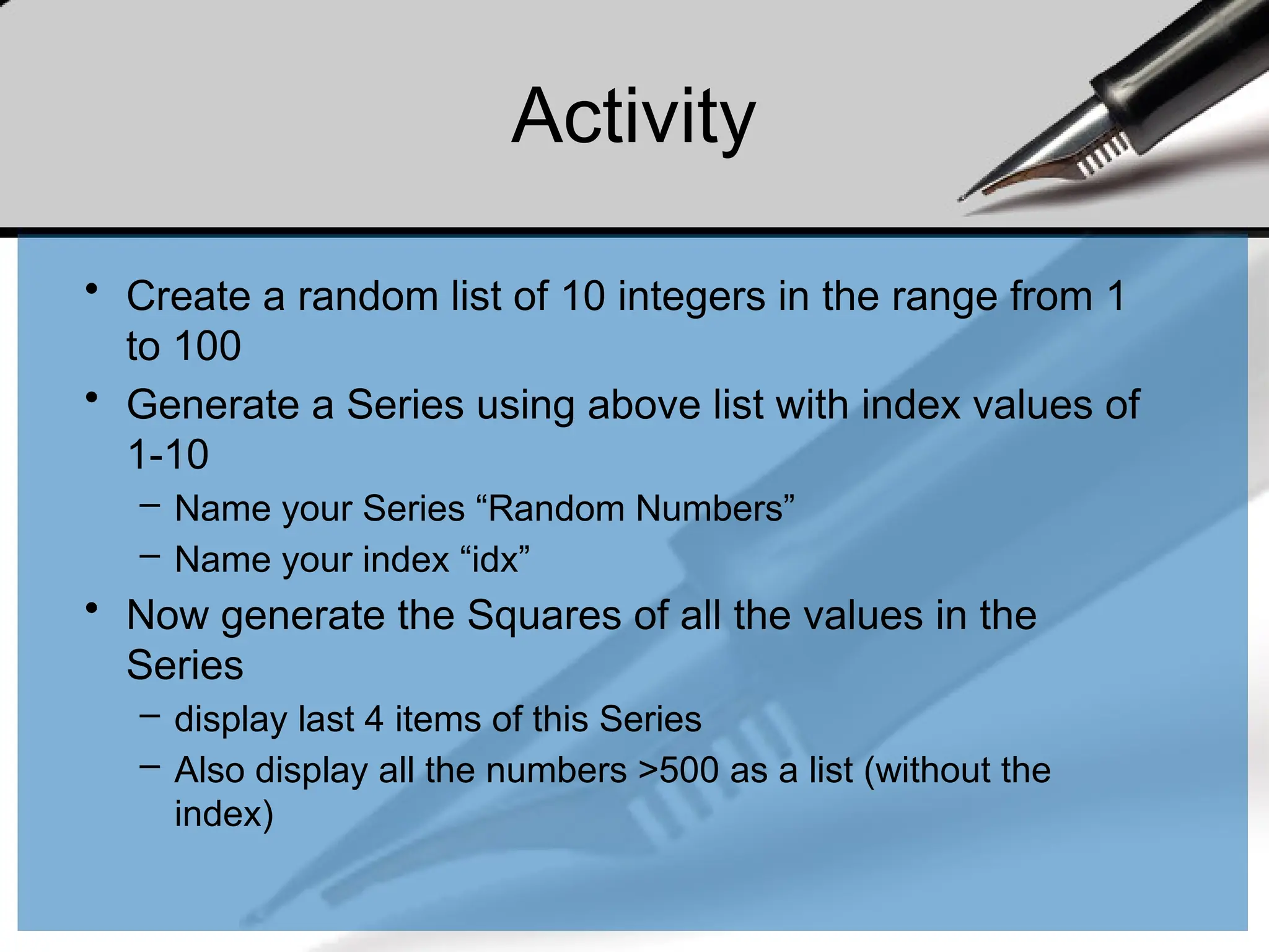
![DataFrame
• A DataFrame is a tabular data structure comprised of rows and
columns, akin to a spreadsheet or database table.
• It can be treated as an ordered collection of columns
– Each column can be a different data type
– Have both row and column indices
data = {'state': ['Ohio', 'Ohio', 'Ohio', 'Nevada', 'Nevada'],
'year': [2000, 2001, 2002, 2001, 2002],
'pop': [1.5, 1.7, 3.6, 2.4, 2.9]}
frame = DataFrame(data)
print(frame)
#output
state year pop
0 Ohio 2000 1.5
1 Ohio 2001 1.7
2 Ohio 2002 3.6
3 Nevada 2001 2.4
4 Nevada 2002 2.9](https://image.slidesharecdn.com/dalecture1introduction-250915234621-3db310b6/75/DATA-ANALYSIS_Lecture-1-Introduction-pptx-148-2048.jpg)
![DataFrame – specifying
columns and indices
• Order of columns/rows can be specified.
• Columns not in data will have NaN.
frame2 = DataFrame(data, columns=['year', 'state', 'pop', 'debt'], index=['A', 'B', 'C', 'D', 'E'])
Print(frame2)
year state pop debt
A 2000 Ohio 1.5 NaN
B 2001 Ohio 1.7 NaN
C 2002 Ohio 3.6 NaN
D 2001 Nevada 2.4 NaN
E 2002 Nevada 2.9 NaN
Same order
Initialized with NaN](https://image.slidesharecdn.com/dalecture1introduction-250915234621-3db310b6/75/DATA-ANALYSIS_Lecture-1-Introduction-pptx-149-2048.jpg)
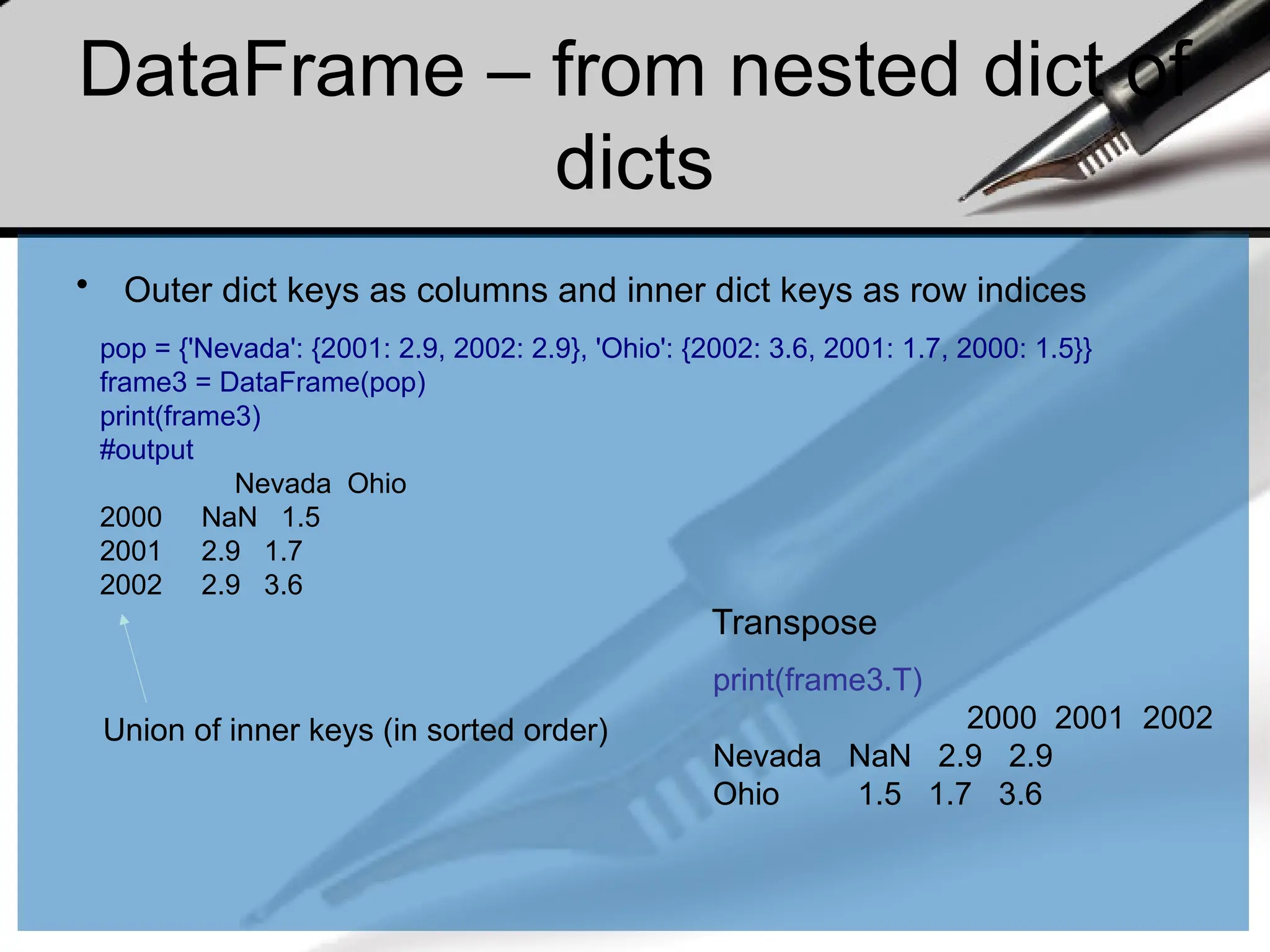
![DataFrame – index, columns,
values
frame3.index.name = 'year'
frame3.columns.name='state‘
print(frame3)
state Nevada Ohio
year
2000 NaN 1.5
2001 2.9 1.7
2002 2.9 3.6
print(frame3.index)
Int64Index([2000, 2001, 2002], dtype='int64', name='year')
print(frame3.columns)
Index(['Nevada', 'Ohio'], dtype='object', name='state')
print(frame3.values)
[[nan 1.5]
[2.9 1.7]
[2.9 3.6]]](https://image.slidesharecdn.com/dalecture1introduction-250915234621-3db310b6/75/DATA-ANALYSIS_Lecture-1-Introduction-pptx-151-2048.jpg)
![DataFrame – retrieving a
column
• A column in a DataFrame can be retrieved as a Series
by dict-like notation or as attribute
data = {'state': ['Ohio', 'Ohio', 'Ohio', 'Nevada', 'Nevada'],
'year': [2000, 2001, 2002, 2001, 2002],
'pop': [1.5, 1.7, 3.6, 2.4, 2.9]}
frame = DataFrame(data)
print(frame['state'])
0 Ohio
1 Ohio
2 Ohio
3 Nevada
4 Nevada
Name: state, dtype: object
print(frame.state)
0 Ohio
1 Ohio
2 Ohio
3 Nevada
4 Nevada
Name: state, dtype: object](https://image.slidesharecdn.com/dalecture1introduction-250915234621-3db310b6/75/DATA-ANALYSIS_Lecture-1-Introduction-pptx-152-2048.jpg)
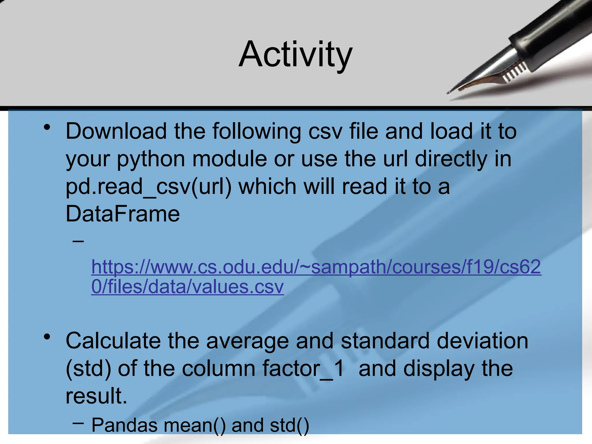
![DataFrame – getting rows
• loc for using indexes and iloc for using positions
– loc gets rows (or columns) with particular labels from the index.
– iloc gets rows (or columns) at particular positions in the index (so it only takes integers).
data = {'state': ['Ohio', 'Ohio', 'Ohio', 'Nevada', 'Nevada'],
'year': [2000, 2001, 2002, 2001, 2002],
'pop': [1.5, 1.7, 3.6, 2.4, 2.9]}
frame2 = DataFrame(data, columns=['year', 'state', 'pop', 'debt'], index=['A', 'B', 'C', 'D', 'E'])
print(frame2)
year state pop debt
A 2000 Ohio 1.5 NaN
B 2001 Ohio 1.7 NaN
C 2002 Ohio 3.6 NaN
D 2001 Nevada 2.4 NaN
E 2002 Nevada 2.9 NaN
print(frame2.loc['A'])
year 2000
state Ohio
pop 1.5
debt NaN
Name: A, dtype: object
print(frame2.loc[['A', 'B']])
year state pop debt
A 2000 Ohio 1.5 NaN
B 2001 Ohio 1.7 NaN
print(frame2.loc['A':'E',
['state','pop']])
state pop
A Ohio 1.5
B Ohio 1.7
C Ohio 3.6
D Nevada 2.4
E Nevada 2.9
print(frame2.iloc[1:3])
year state pop debt
B 2001 Ohio 1.7 NaN
C 2002 Ohio 3.6 NaN
print(frame2.iloc[:,1:3])
state pop
A Ohio 1.5
B Ohio 1.7
C Ohio 3.6
D Nevada 2.4
E Nevada 2.9](https://image.slidesharecdn.com/dalecture1introduction-250915234621-3db310b6/75/DATA-ANALYSIS_Lecture-1-Introduction-pptx-154-2048.jpg)
![DataFrame – modifying
columns
frame2['debt'] = 0
print(frame2)
year state pop debt
A 2000 Ohio 1.5 0
B 2001 Ohio 1.7 0
C 2002 Ohio 3.6 0
D 2001 Nevada 2.4 0
E 2002 Nevada 2.9 0
frame2['debt'] = range(5)
print(frame2)
year state pop debt
A 2000 Ohio 1.5 0
B 2001 Ohio 1.7 1
C 2002 Ohio 3.6 2
D 2001 Nevada 2.4 3
E 2002 Nevada 2.9 4
val = Series([10, 10, 10], index = ['A', 'C', 'D'])
frame2['debt'] = val
print(frame2)
year state pop debt
A 2000 Ohio 1.5 10.0
B 2001 Ohio 1.7 NaN
C 2002 Ohio 3.6 10.0
D 2001 Nevada 2.4 10.0
E 2002 Nevada 2.9 NaN
Rows or individual elements can be
modified similarly. Using loc or iloc.](https://image.slidesharecdn.com/dalecture1introduction-250915234621-3db310b6/75/DATA-ANALYSIS_Lecture-1-Introduction-pptx-155-2048.jpg)
![DataFrame:removing columns
del frame2['debt']
print(frame2)
year state pop
A 2000 Ohio 1.5
B 2001 Ohio 1.7
C 2002 Ohio 3.6
D 2001 Nevada 2.4
E 2002 Nevada 2.9](https://image.slidesharecdn.com/dalecture1introduction-250915234621-3db310b6/75/DATA-ANALYSIS_Lecture-1-Introduction-pptx-156-2048.jpg)
![More on DataFrame indexing
import numpy as np
data = np.arange(9).reshape(3,3)
print(data)
[[0 1 2]
[3 4 5]
[6 7 8]]
frame = DataFrame(data, index=['r1', 'r2', 'r3'], columns=['c1', 'c2', 'c3'])
print(frame)
c1 c2 c3
r1 0 1 2
r2 3 4 5
r3 6 7 8
print(frame['c1'])
r1 0
r2 3
r3 6
Name: c1, dtype: int32
print(frame['c1']['r1'])
0
print(frame[['c1', 'c3']])
c1 c3
r1 0 2
r2 3 5
r3 6 8
print(frame.loc['r1'])
c1 0
c2 1
c3 2
Name: r1, dtype: int32
print(frame.loc[['r1','r3']])
c1 c2 c3
r1 0 1 2
r3 6 7 8
print(frame[:2])
c1 c2 c3
r1 0 1 2
r2 3 4 5
print(frame.iloc[:2])
c1 c2 c3
r1 0 1 2
r2 3 4 5
Row slices](https://image.slidesharecdn.com/dalecture1introduction-250915234621-3db310b6/75/DATA-ANALYSIS_Lecture-1-Introduction-pptx-157-2048.jpg)
![More on DataFrame indexing
print(frame.loc[['r1', 'r2'], ['c1', 'c2']])
c1 c2
r1 0 1
r2 3 4
print(frame.iloc[:2,:2])
c1 c2
r1 0 1
r2 3 4
v = DataFrame(np.arange(9).reshape(3,3), index=['a', 'a', 'b'], columns=['c1','c2','c3'])
print(v)
c1 c2 c3
a 0 1 2
a 3 4 5
b 6 7 8
print(v.loc['a'])
c1 c2 c3
a 0 1 2
a 3 4 5
Duplicated keys
print(frame.loc['r1':'r3', 'c1':'c3'])
c1 c2 c3
r1 0 1 2
r2 3 4 5
r3 6 7 8](https://image.slidesharecdn.com/dalecture1introduction-250915234621-3db310b6/75/DATA-ANALYSIS_Lecture-1-Introduction-pptx-158-2048.jpg)
![More on DataFrame indexing
print(frame)
c1 c2 c3
r1 0 1 2
r2 3 4 5
r3 6 7 8
print(frame <3)
c1 c2 c3
r1 True True True
r2 False False False
r3 False False False
print(frame[frame['c1']>0])
c1 c2 c3
r2 3 4 5
r3 6 7 8
print(frame['c1']>0)
r1 False
r2 True
r3 True
Name: c1, dtype: bool
frame[frame<3] = 3
print(frame)
c1 c2 c3
r1 3 3 3
r2 3 4 5
r3 6 7 8](https://image.slidesharecdn.com/dalecture1introduction-250915234621-3db310b6/75/DATA-ANALYSIS_Lecture-1-Introduction-pptx-159-2048.jpg)
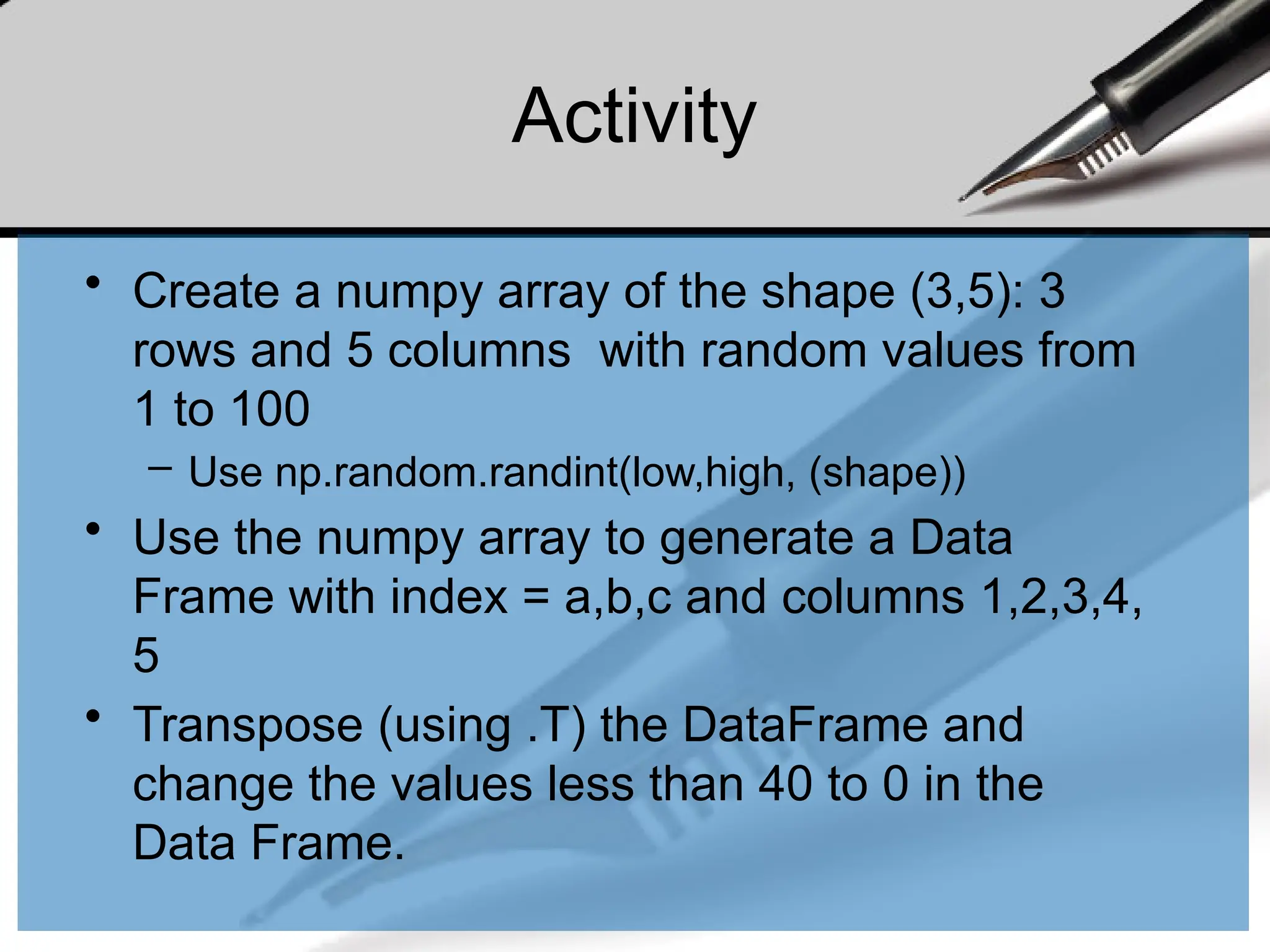
![Removing rows/columns
print(frame)
c1 c2 c3
r1 0 1 2
r2 3 4 5
r3 6 7 8
print(frame.drop(['r1']))
c1 c2 c3
r2 3 4 5
r3 6 7 8
print(frame.drop(['r1','r3']))
c1 c2 c3
r2 3 4 5
print(frame.drop(['c1'], axis=1))
c2 c3
r1 1 2
r2 4 5
r3 7 8
This returns a new object](https://image.slidesharecdn.com/dalecture1introduction-250915234621-3db310b6/75/DATA-ANALYSIS_Lecture-1-Introduction-pptx-161-2048.jpg)
![Reindexing
• Alter the order of rows/columns of a DataFrame or order of a series
according to new index
frame2 = frame.reindex(columns=['c2', 'c3', 'c1'])
print(frame2)
c2 c3 c1
r1 1 2 0
r2 4 5 3
r3 7 8 6
frame2 = frame.reindex(['r1', 'r3', 'r2', 'r4'])
c1 c2 c3
r1 0.0 1.0 2.0
r3 6.0 7.0 8.0
r2 3.0 4.0 5.0
r4 NaN NaN NaN
This returns a new object](https://image.slidesharecdn.com/dalecture1introduction-250915234621-3db310b6/75/DATA-ANALYSIS_Lecture-1-Introduction-pptx-162-2048.jpg)
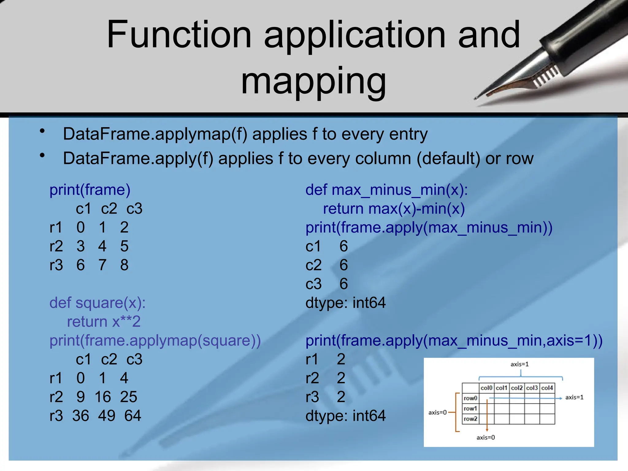
![Function application and
mapping
def max_min(x):
return Series([max(x), min(x)], index=['max', 'min'])
print(frame.apply(max_min))
c1 c2 c3
max 6 7 8
min 0 1 2](https://image.slidesharecdn.com/dalecture1introduction-250915234621-3db310b6/75/DATA-ANALYSIS_Lecture-1-Introduction-pptx-164-2048.jpg)
![Other DataFrame functions
• sort_index()
frame.index=['A', 'C', 'B'];
frame.columns=['b','a','c'];
print(frame)
b a c
A 0 1 2
C 3 4 5
B 6 7 8
print(frame.sort_index())
b a c
A 0 1 2
B 6 7 8
C 3 4 5
print(frame.sort_index(axis=1))
a b c
A 1 0 2
C 4 3 5
B 7 6 8
frame = DataFrame(np.random.randint(0, 10, 9).reshape(3,-1),
index=['r1', 'r2', 'r3'], columns=['c1', 'c2', 'c3'])
print(frame)
c1 c2 c3
r1 6 9 0
r2 8 2 9
r3 8 0 6
print(frame.sort_values(by='c1'))
c1 c2 c3
r1 6 9 0
r2 8 2 9
r3 8 0 6
print(frame.sort_values(axis=1,by=['r3','r1']))
c2 c3 c1
r1 9 0 6
r2 2 9 8
r3 0 6 8
• sort_values()](https://image.slidesharecdn.com/dalecture1introduction-250915234621-3db310b6/75/DATA-ANALYSIS_Lecture-1-Introduction-pptx-165-2048.jpg)
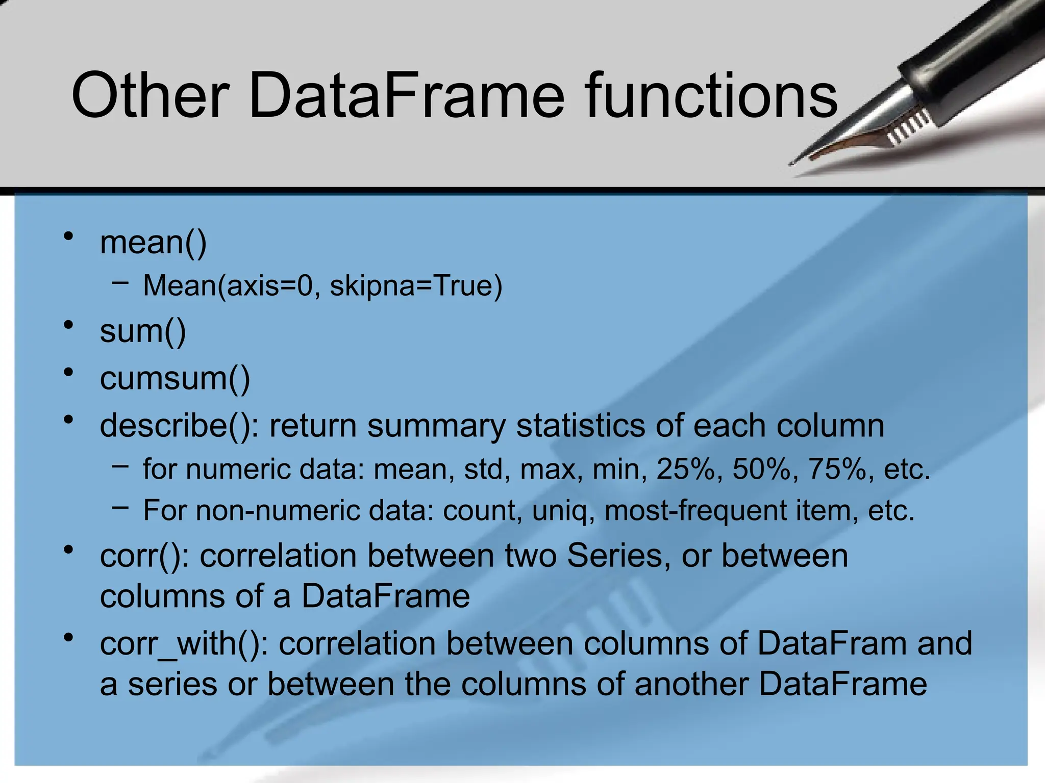
![Handling missing data
• Filtering out missing values
from numpy import nan as NaN
data = Series([1, NaN, 2.5, NaN, 6])
print(data)
0 1.0
1 NaN
2 2.5
3 NaN
4 6.0
dtype: float64
print(data.notnull())
0 True
1 False
2 True
3 False
4 True
dtype: bool
print(data[data.notnull()])
0 1.0
2 2.5
4 6.0
dtype: float64
print(data.dropna())
0 1.0
2 2.5
4 6.0
dtype: float64](https://image.slidesharecdn.com/dalecture1introduction-250915234621-3db310b6/75/DATA-ANALYSIS_Lecture-1-Introduction-pptx-168-2048.jpg)
![Handling missing data
data = DataFrame([[1, 2, 3], [1, NaN, NaN], [NaN, NaN, NaN], [NaN, 4, 5]])
print(data)
0 1 2
0 1.0 2.0 3.0
1 1.0 NaN NaN
2 NaN NaN NaN
3 NaN 4.0 5.0
print(data.dropna())
0 1 2
0 1.0 2.0 3.0
print(data.dropna(how='all'))
0 1 2
0 1.0 2.0 3.0
1 1.0 NaN NaN
3 NaN 4.0 5.0
print(data.dropna(axis=1, how='all'))
0 1 2
0 1.0 2.0 3.0
1 1.0 NaN NaN
2 NaN NaN NaN
3 NaN 4.0 5.0
data[4]=NaN
print(data)
0 1 2 4
0 1.0 2.0 3.0 NaN
1 1.0 NaN NaN NaN
2 NaN NaN NaN NaN
3 NaN 4.0 5.0 NaN
print(data.dropna(axis=1, how='all'))
0 1 2
0 1.0 2.0 3.0
1 1.0 NaN NaN
2 NaN NaN NaN
3 NaN 4.0 5.0](https://image.slidesharecdn.com/dalecture1introduction-250915234621-3db310b6/75/DATA-ANALYSIS_Lecture-1-Introduction-pptx-169-2048.jpg)
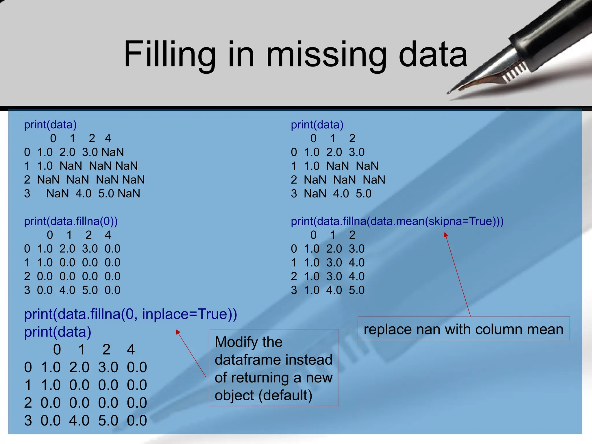
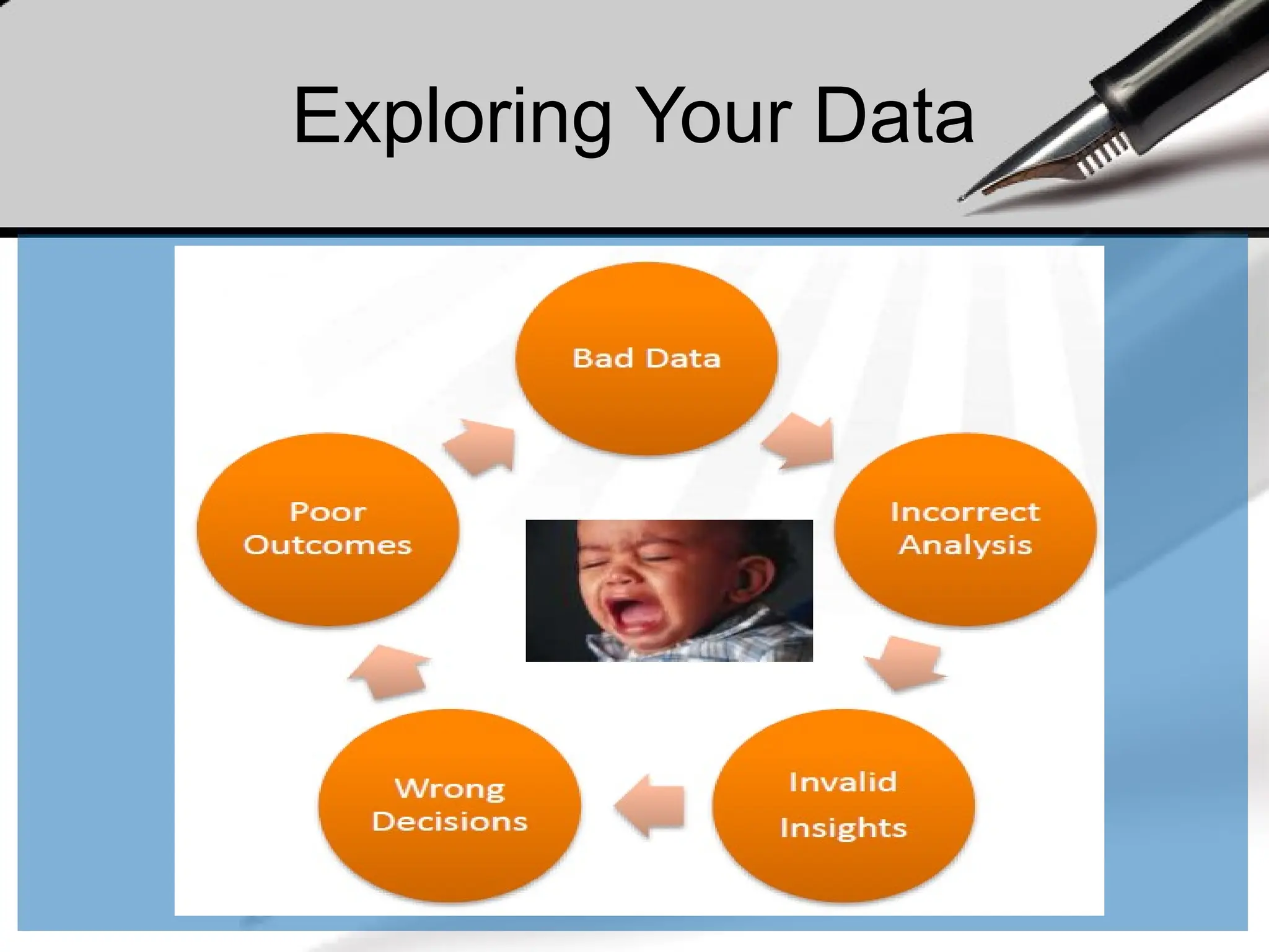
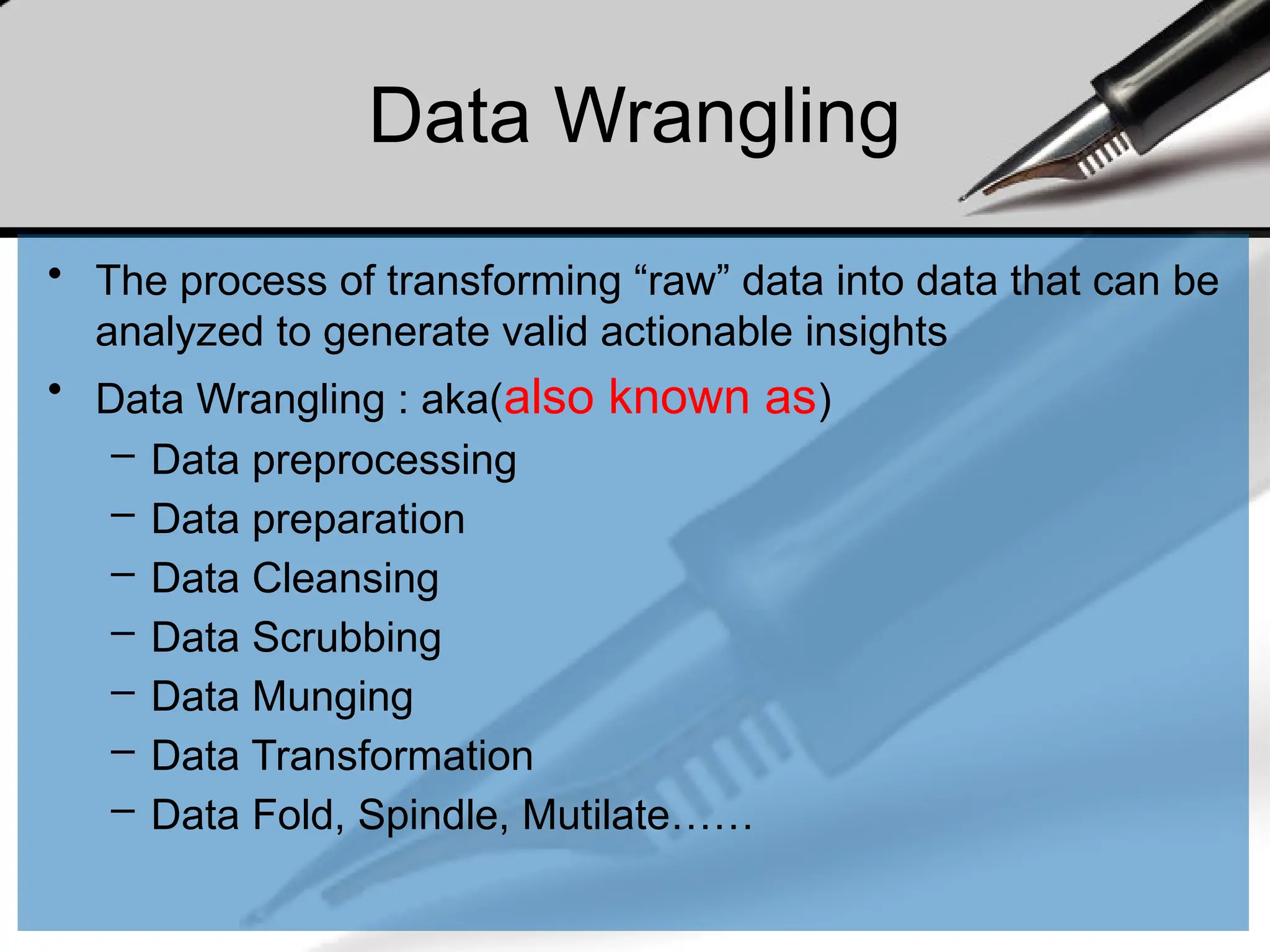
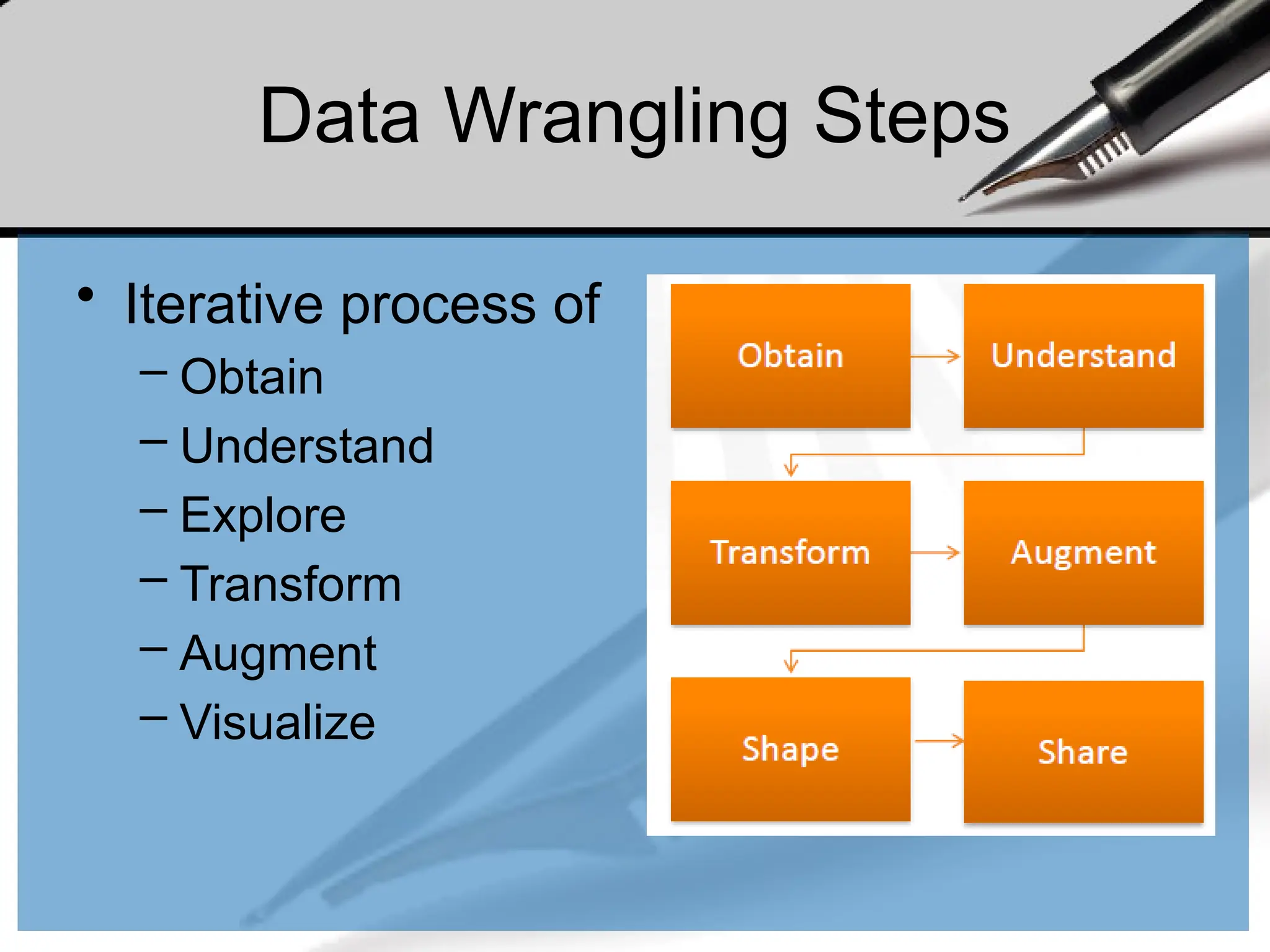
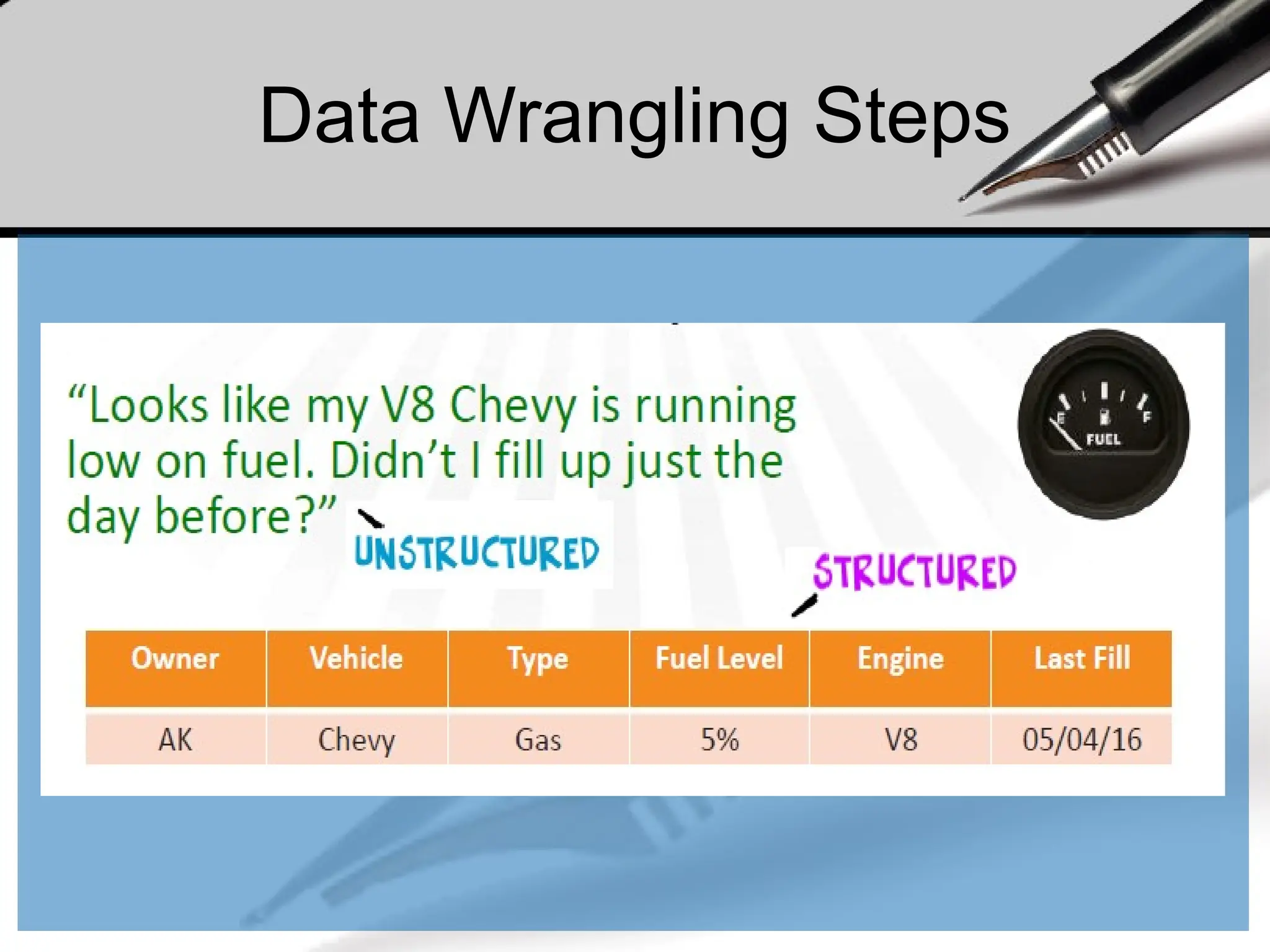
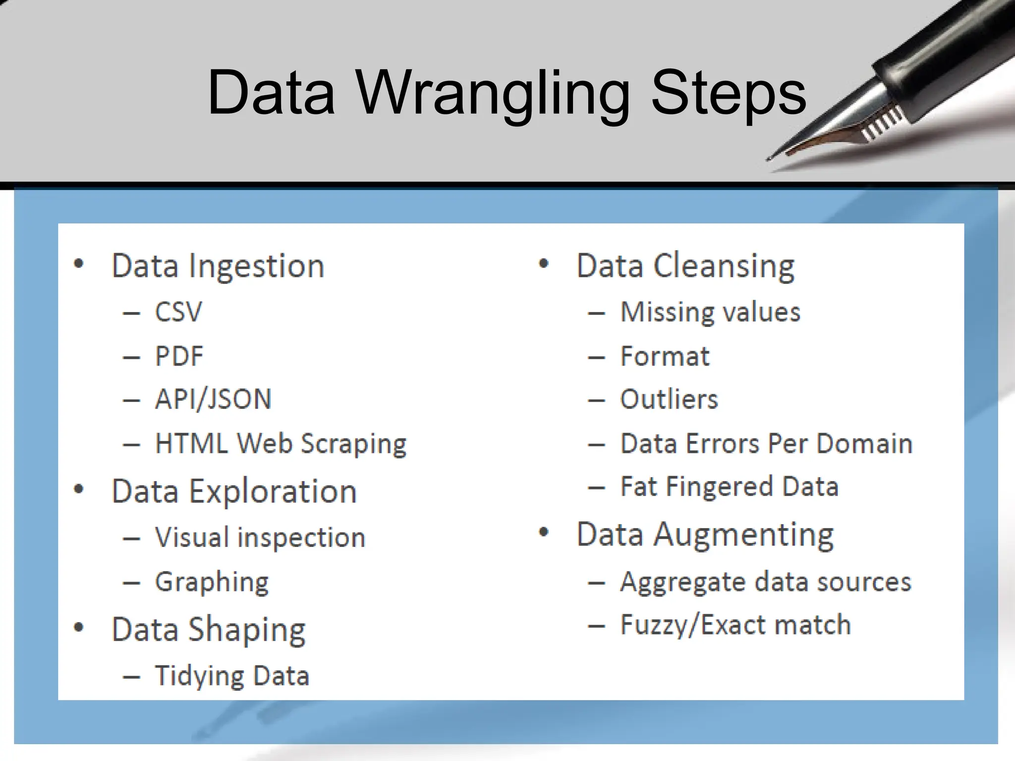

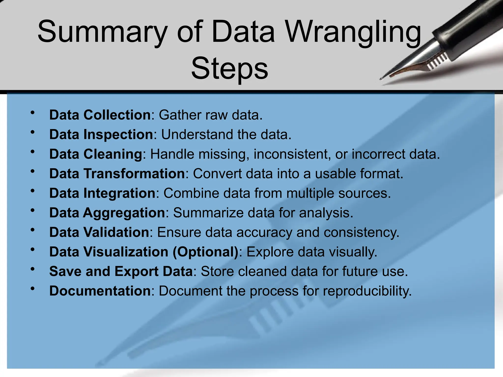
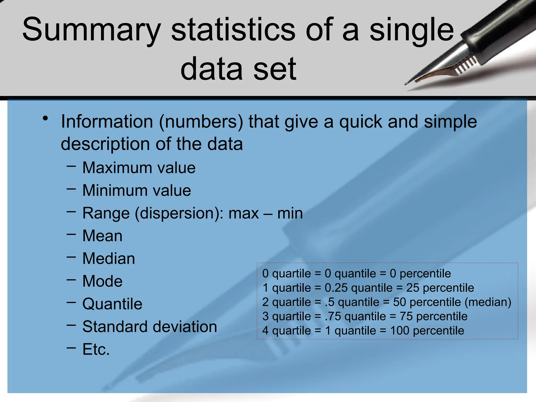
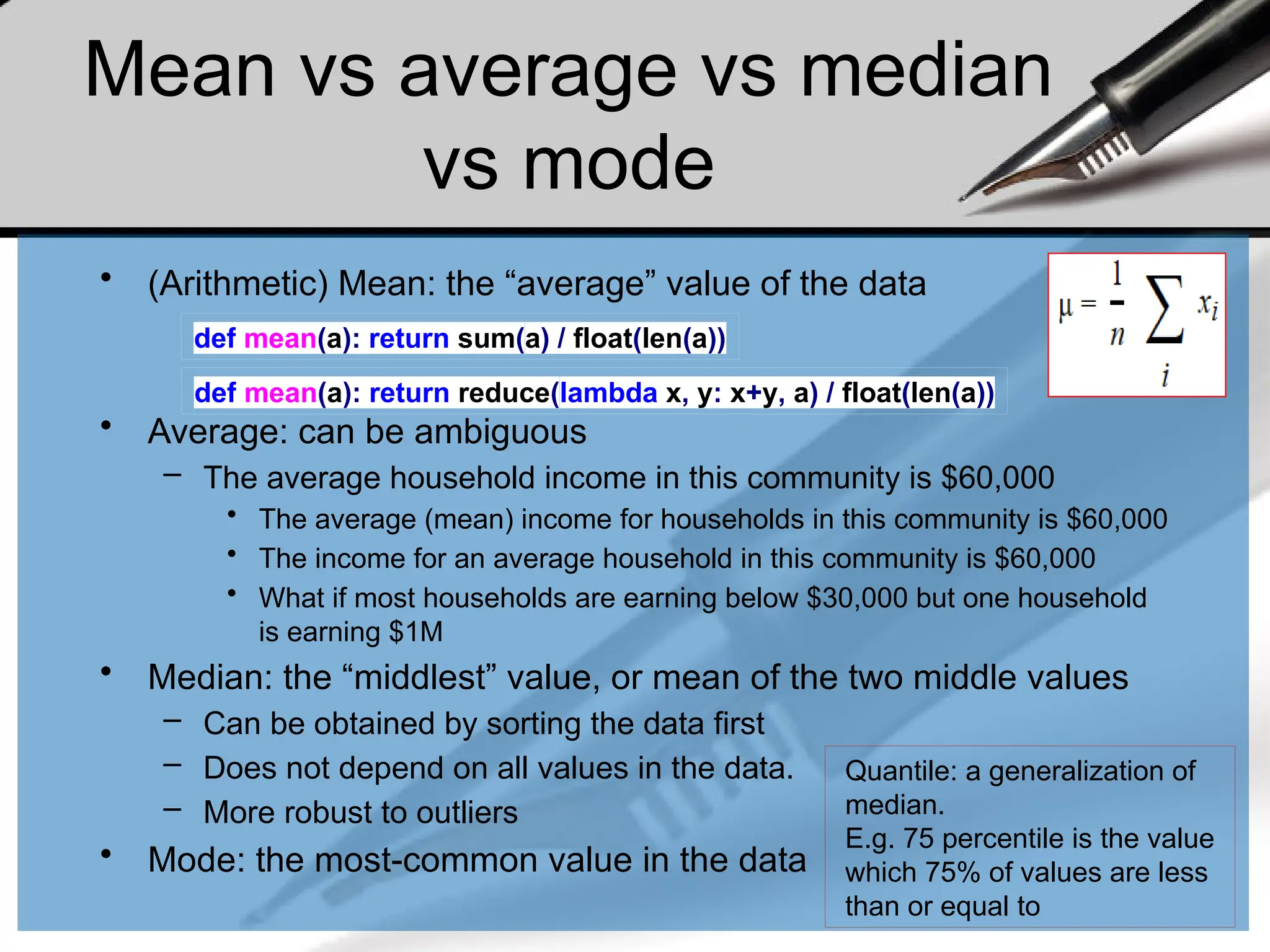
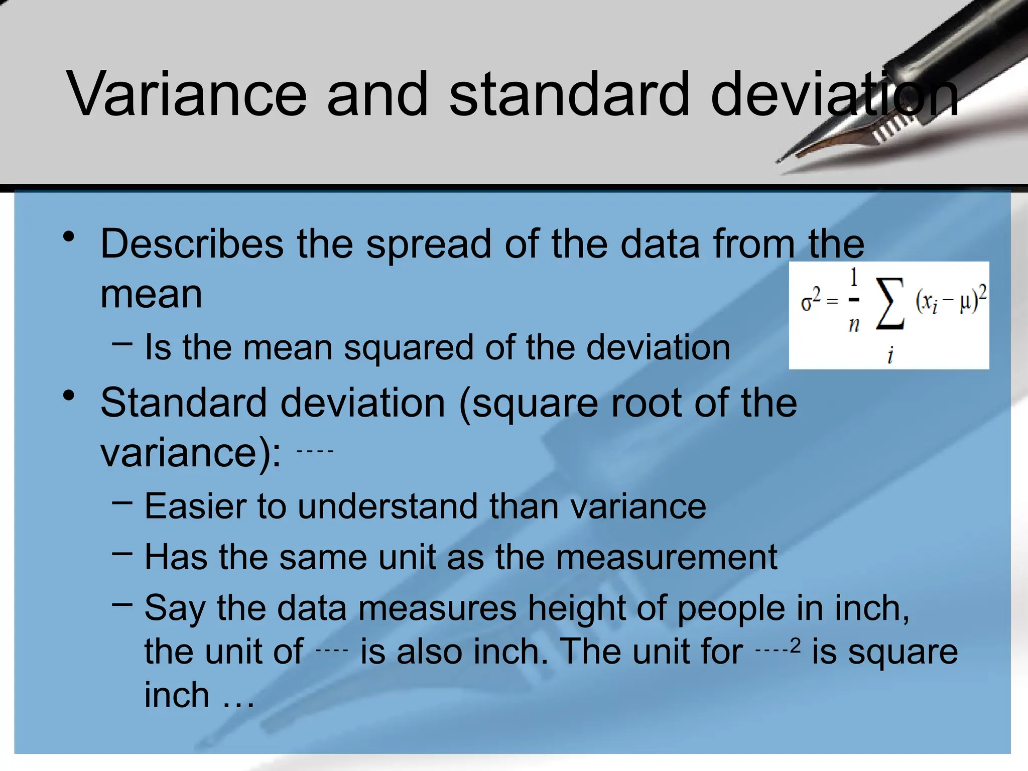

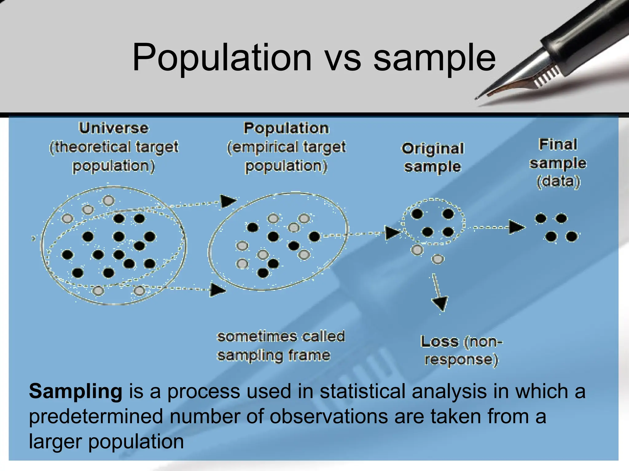
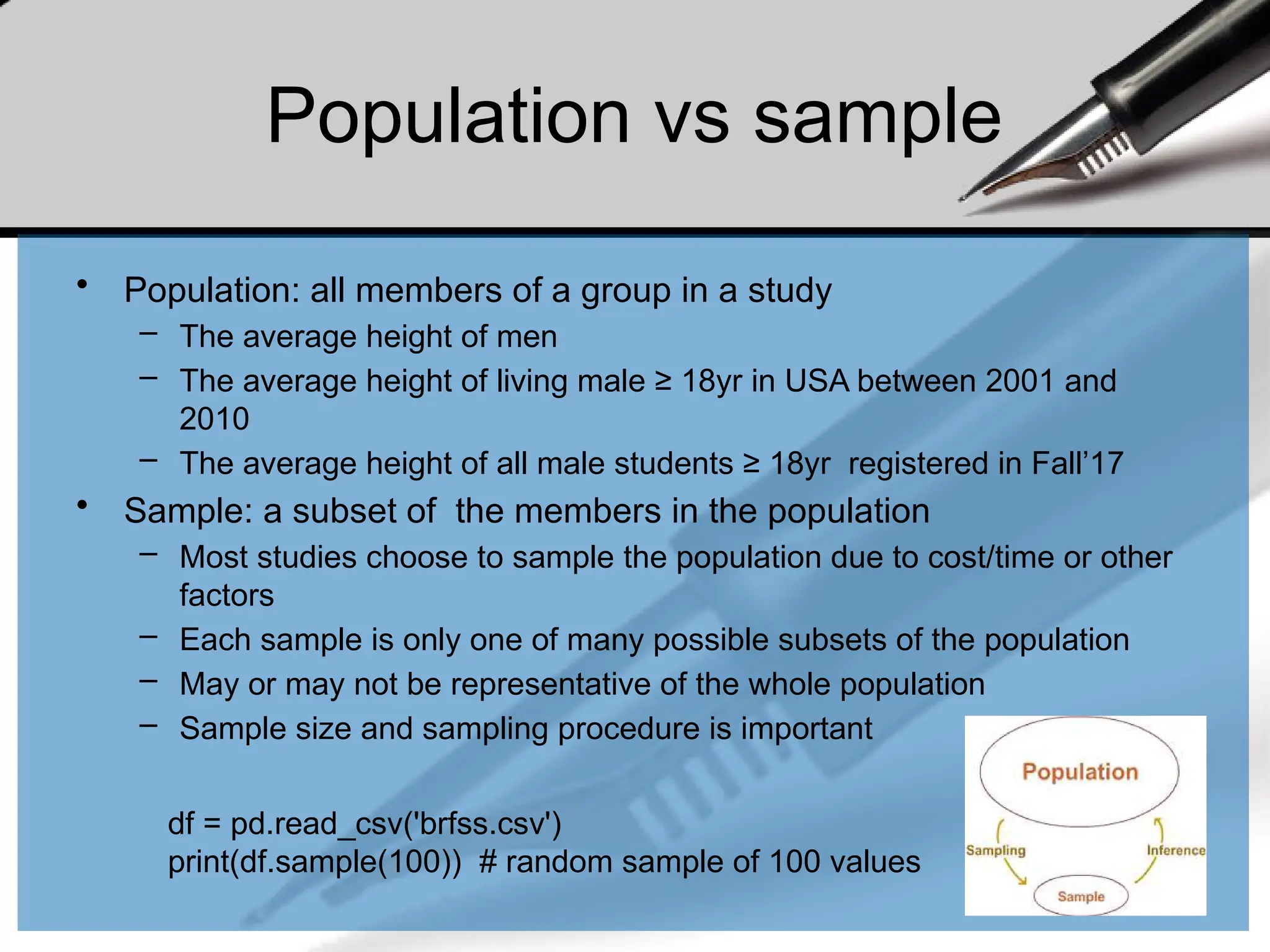
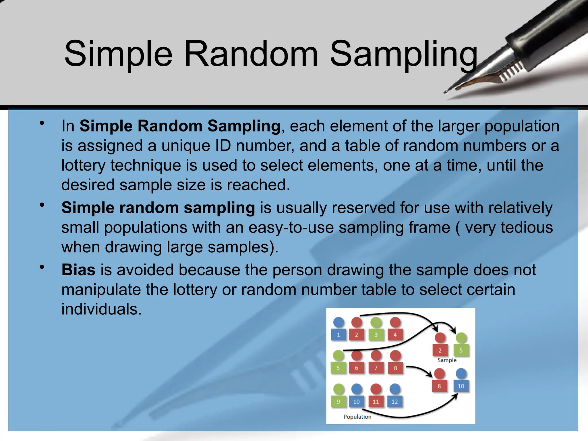
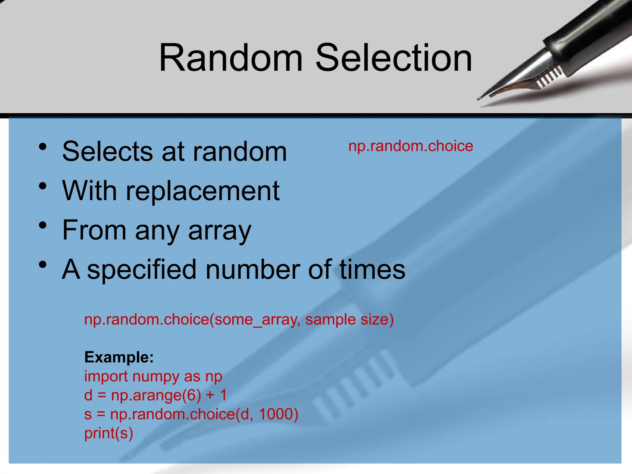
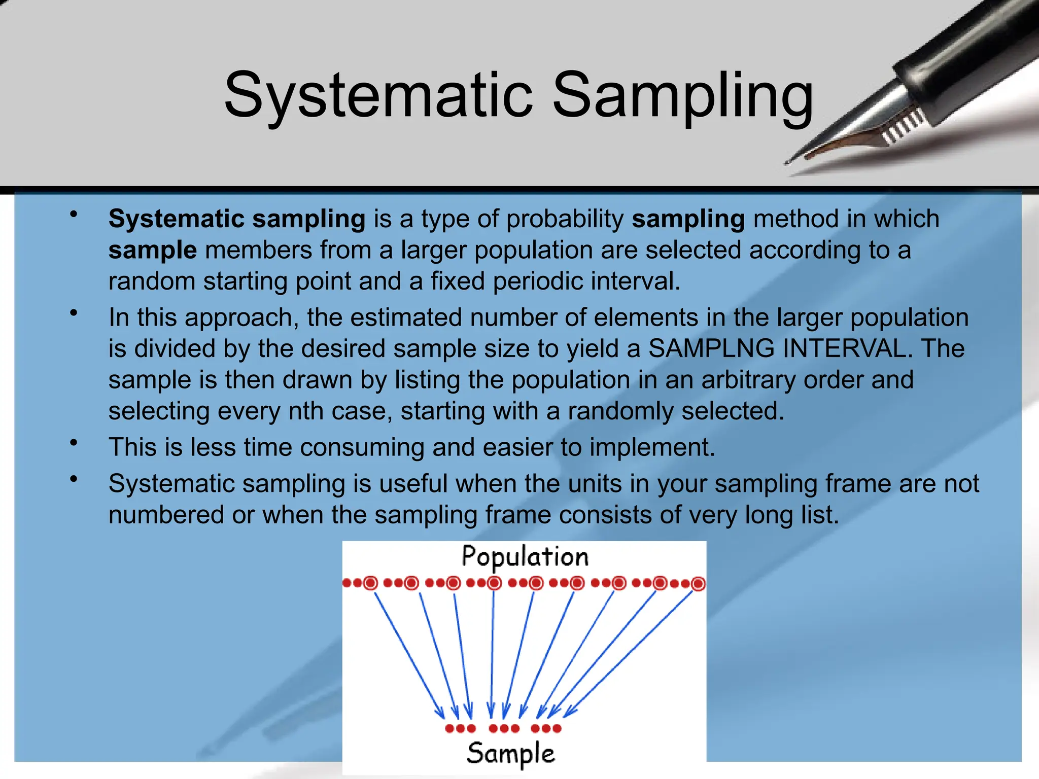
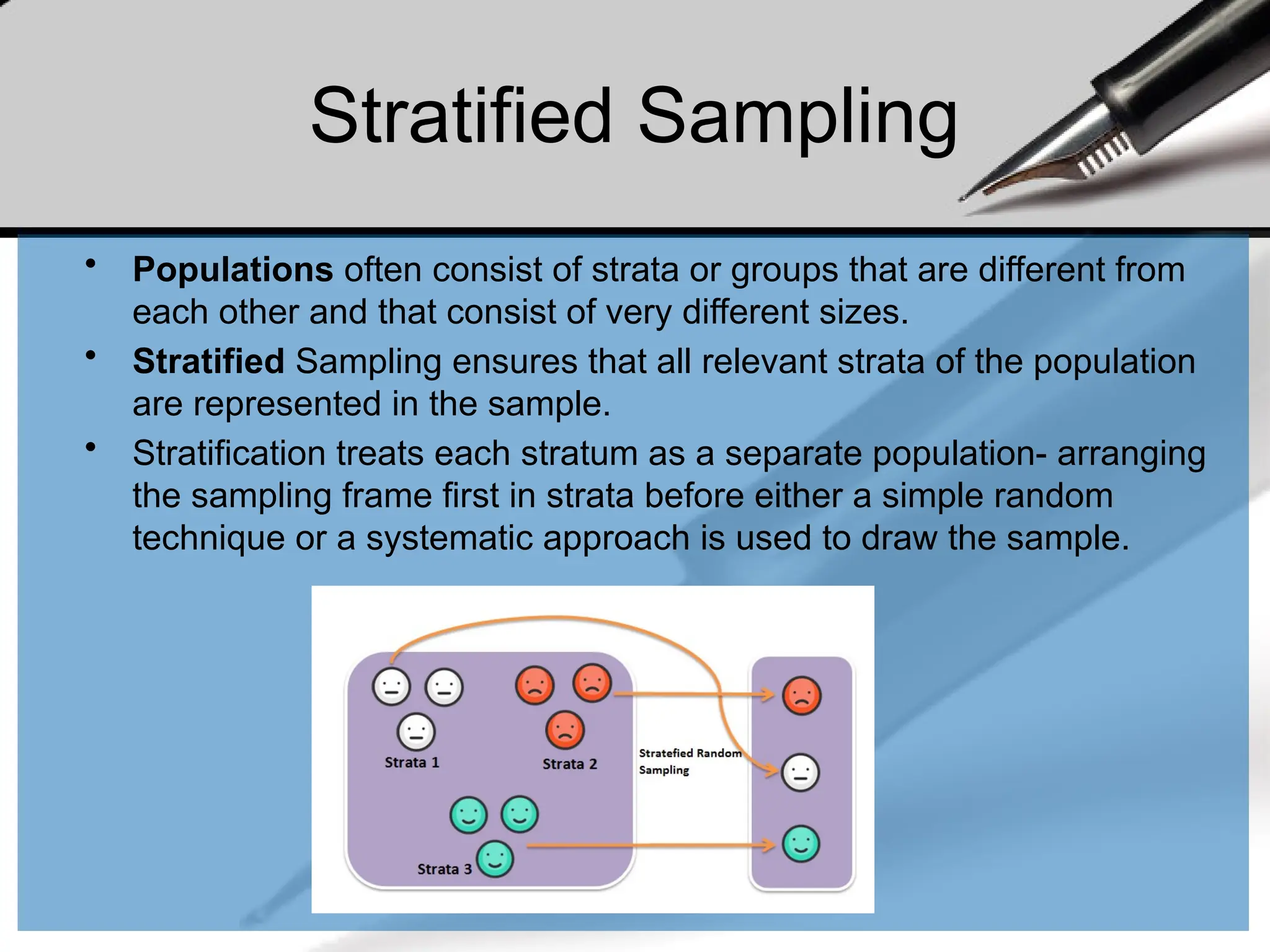
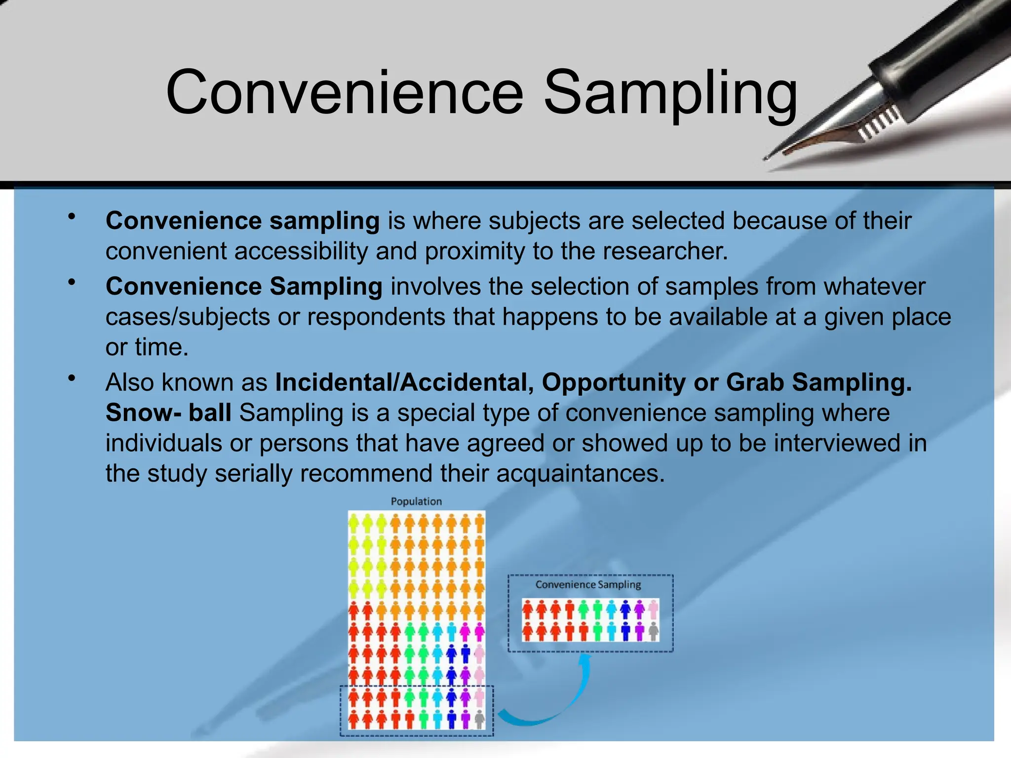
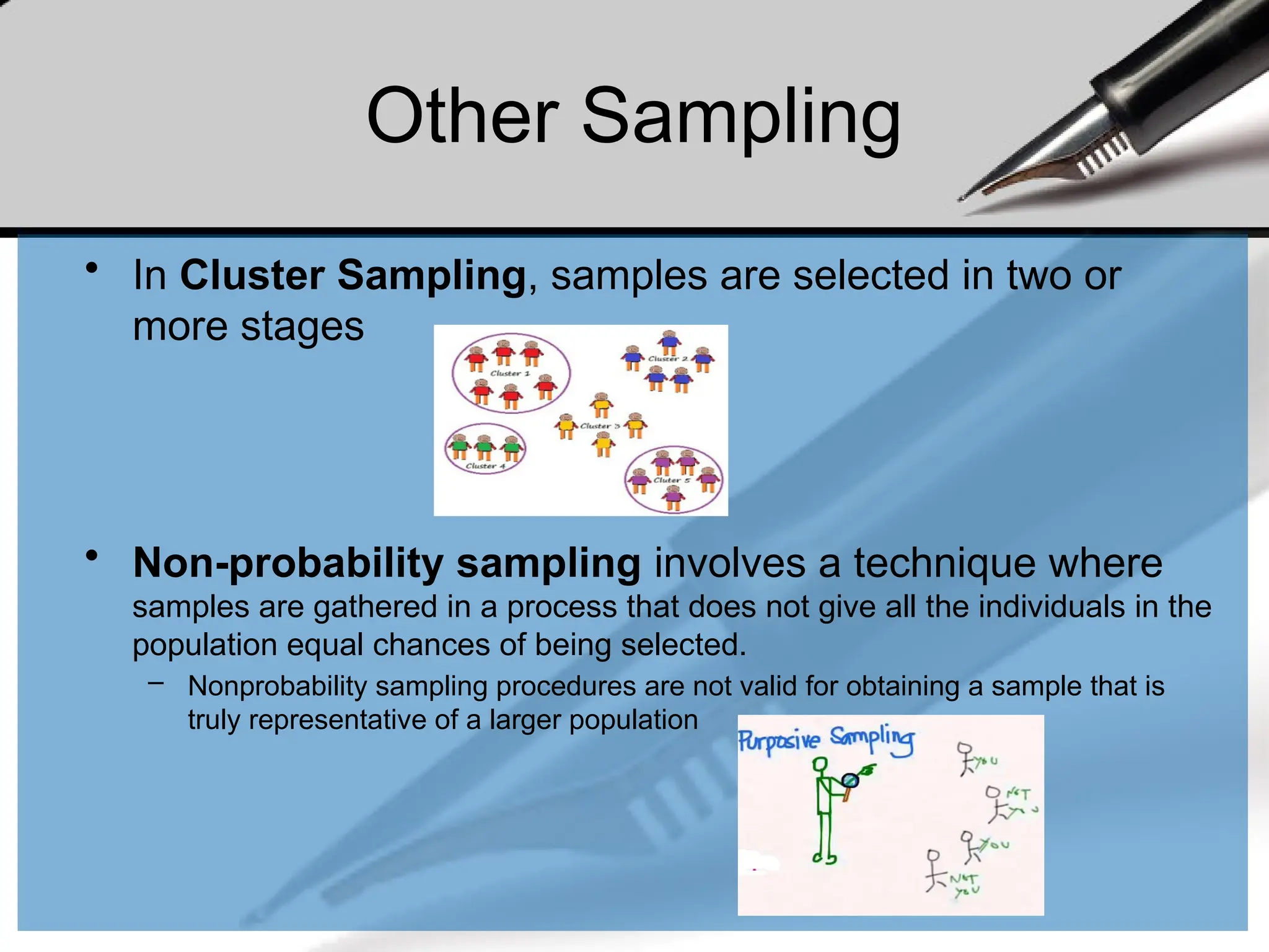
![Exploring Your Data
• Good next step is to create a histogram, in which you
group your data into discrete buckets and count how
many points fall into each bucket:
df = pd.read_csv('brfss.csv', index_col=0)
df['weight2'].hist(bins=100)
A histogram is a plot that lets
you discover, and show, the
underlying frequency
distribution (shape) of a set
of continuous data. This
allows the inspection of the
data for its underlying
distribution (e.g., normal
distribution), outliers,
skewness, etc.](https://image.slidesharecdn.com/dalecture1introduction-250915234621-3db310b6/75/DATA-ANALYSIS_Lecture-1-Introduction-pptx-205-2048.jpg)
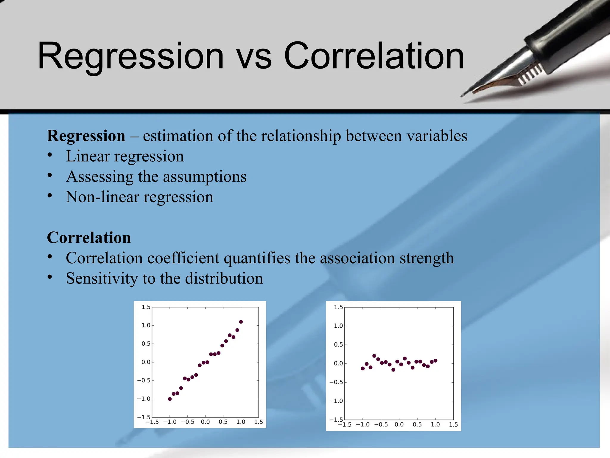
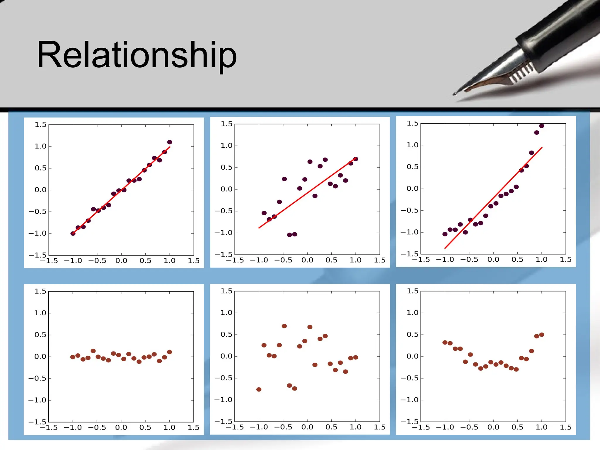
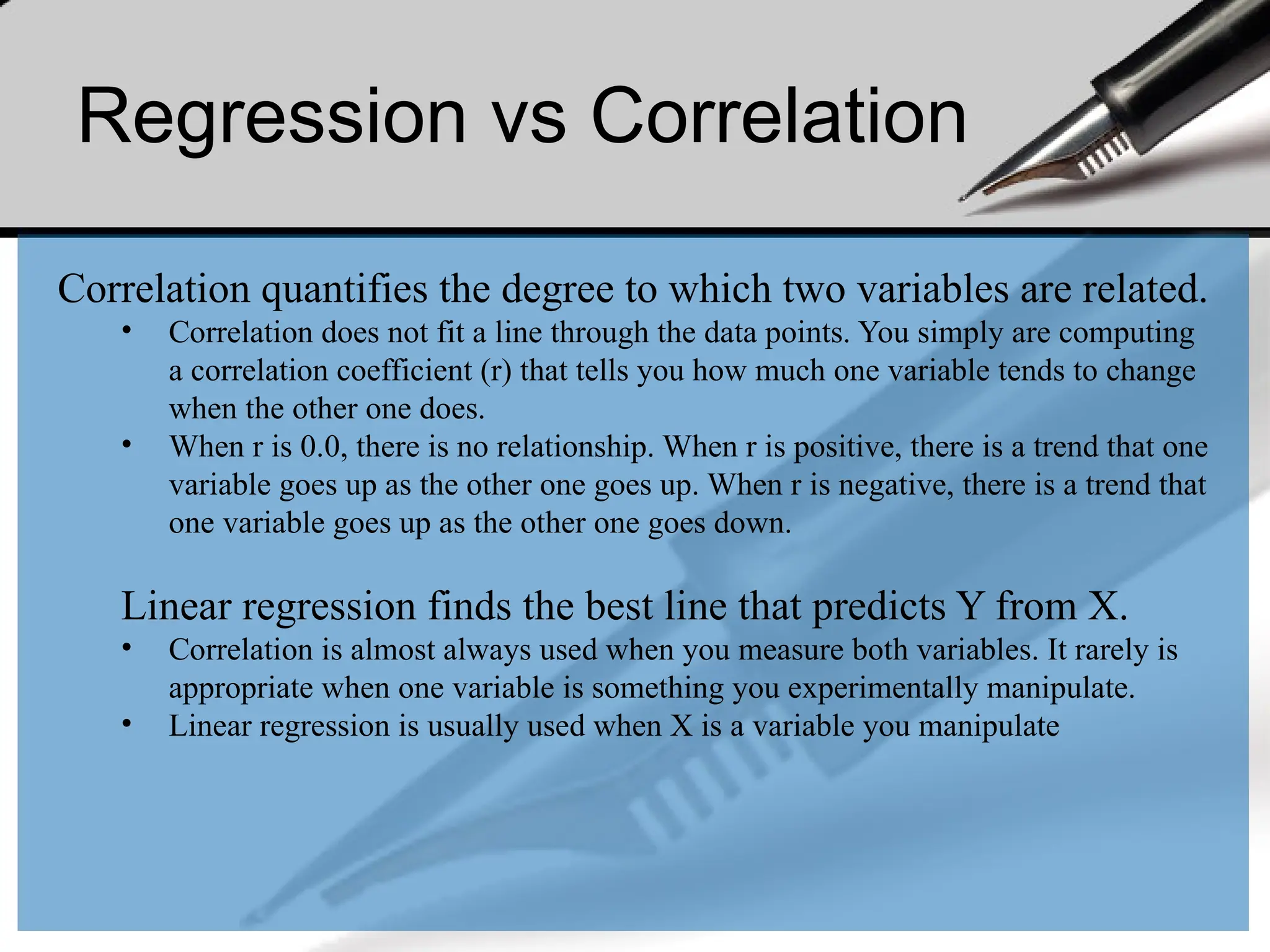
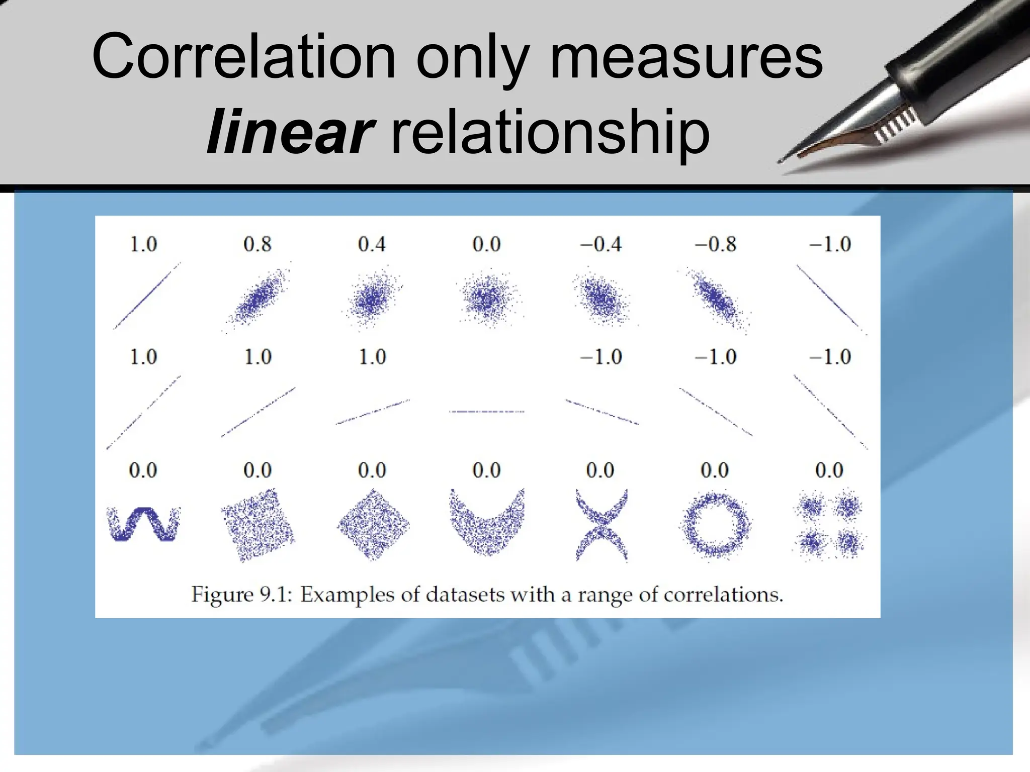
![Feature Matrix
• We can review the relationships between attributes by looking at
the distribution of the interactions of each pair of attributes.
from pandas.tools.plotting import
scatter_matrix
scatter_matrix(df[['weight2', 'wtyrago', 'htm3' ]])
This is a powerful plot from
which a lot of inspiration
about the data can be drawn.
For example, we can see a
possible correlation between
weight and weight year ago](https://image.slidesharecdn.com/dalecture1introduction-250915234621-3db310b6/75/DATA-ANALYSIS_Lecture-1-Introduction-pptx-210-2048.jpg)
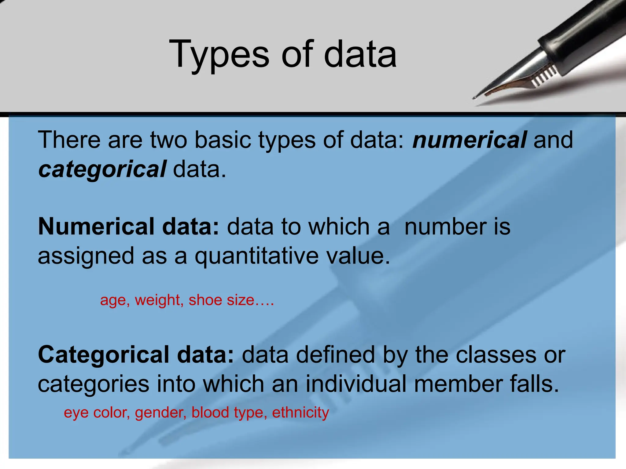
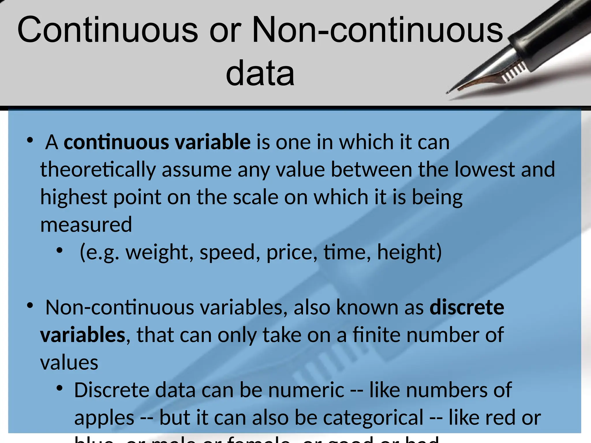
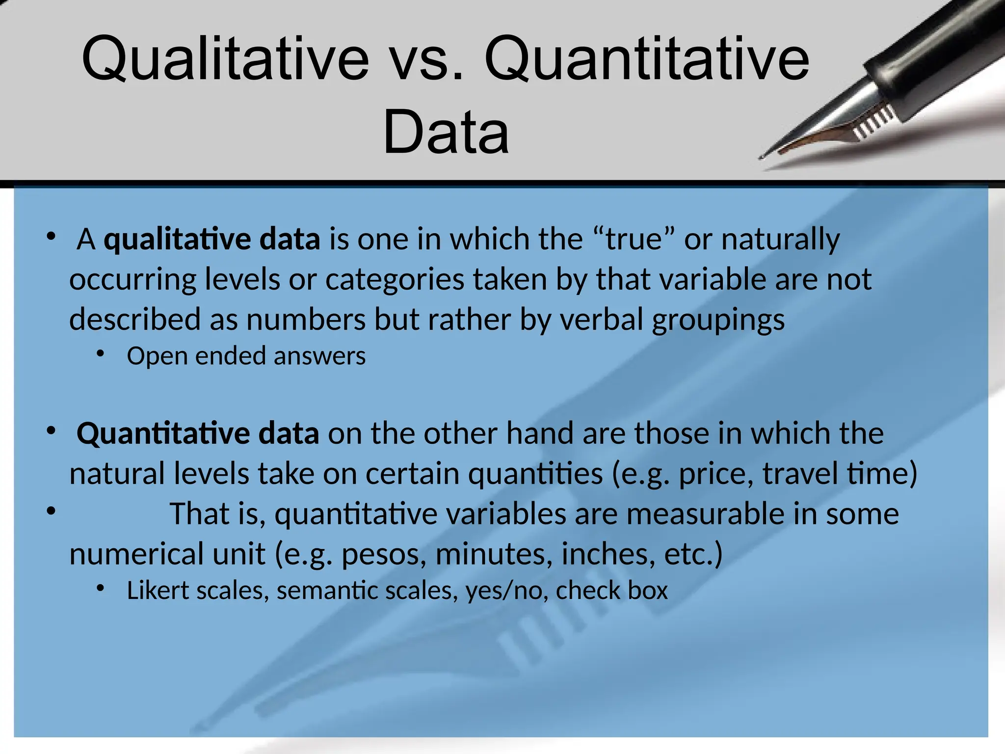
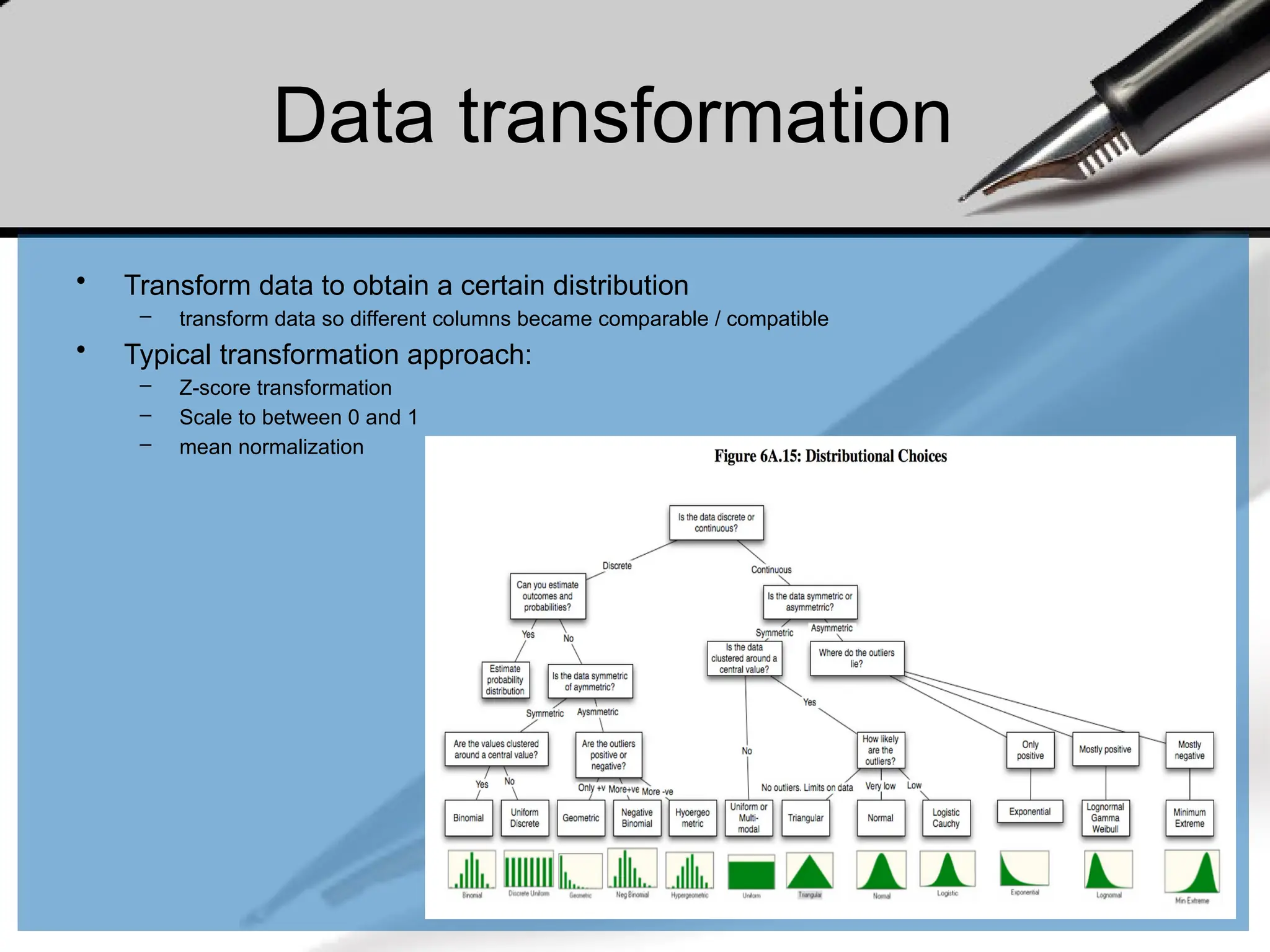
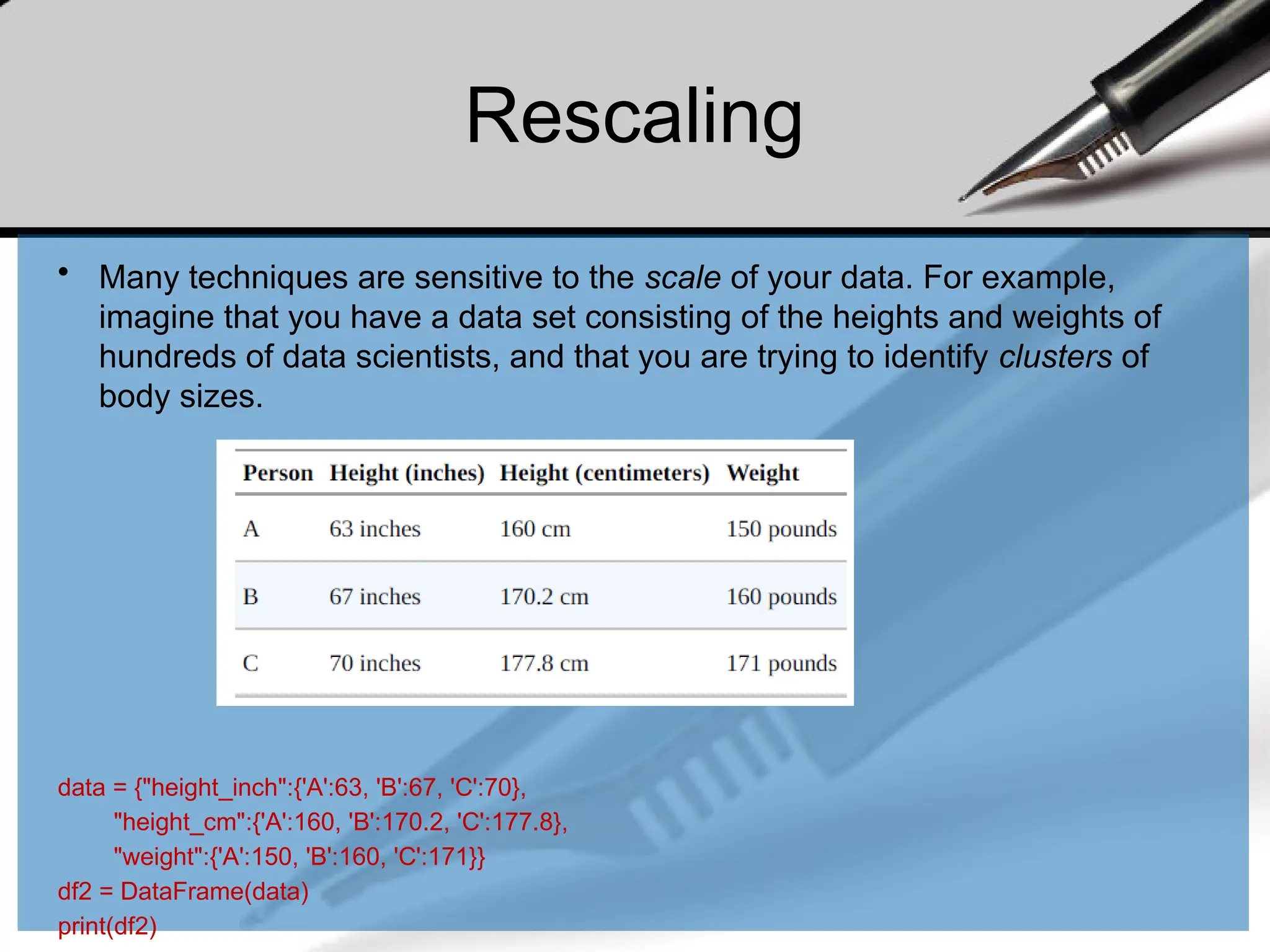
![Why normalization (re-scaling)
height_inch height_cm weight
A 63 160.0 150
B 67 170.2 160
C 70 177.8 171
from scipy.spatial import distance
a = df2.iloc[0, [0,2]]
b = df2.iloc[1, [0,2]]
c = df2.iloc[2, [0,2]]
print("%.2f" % distance.euclidean(a,b)) #10.77
print("%.2f" % distance.euclidean(a,c)) # 22.14
print("%.2f" % distance.euclidean(b,c)) #11.40](https://image.slidesharecdn.com/dalecture1introduction-250915234621-3db310b6/75/DATA-ANALYSIS_Lecture-1-Introduction-pptx-216-2048.jpg)
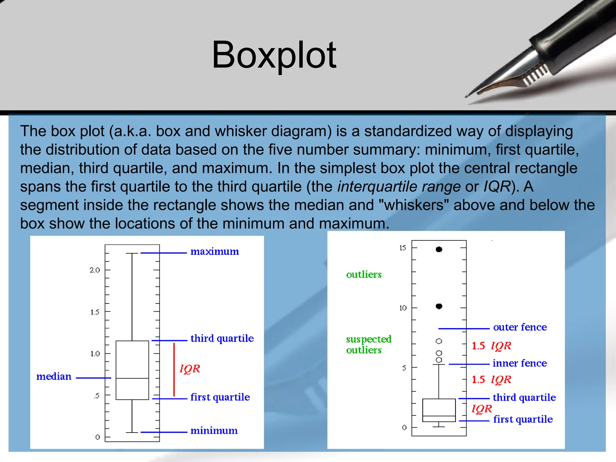
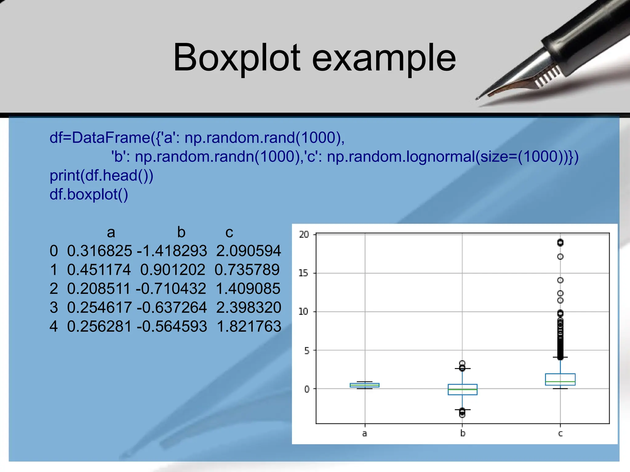
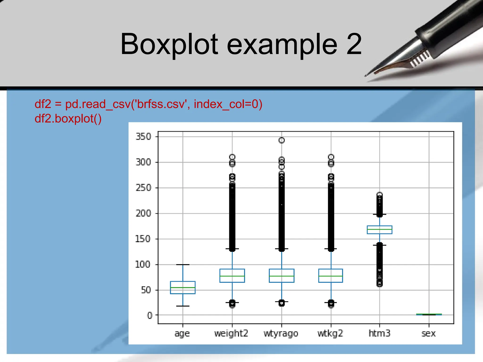
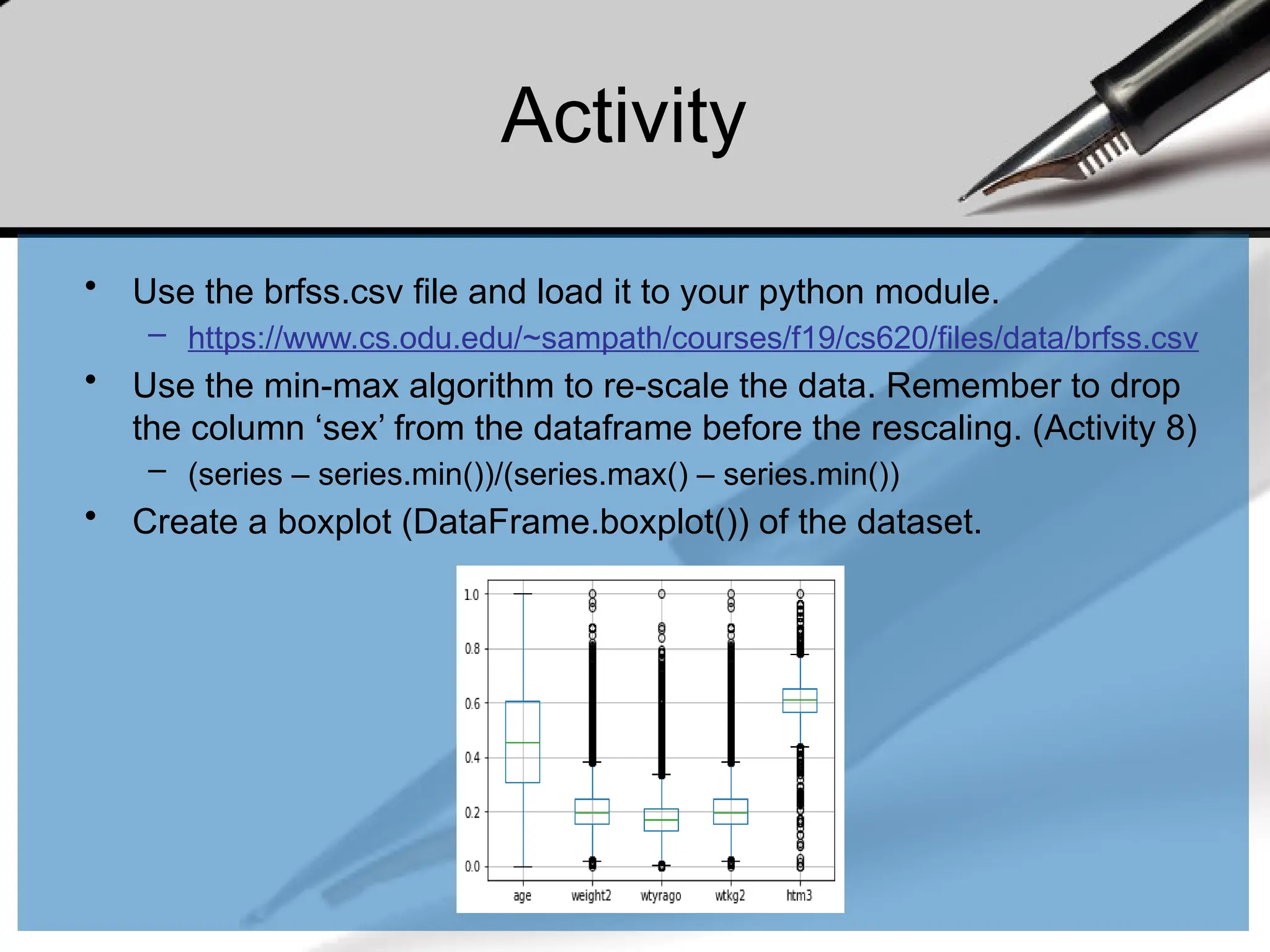
![Z-score transformation
• Z scores, or standard scores, indicate how many standard
deviations an observation is above or below the mean. These
scores are a useful way of putting data from different sources
onto the same scale.
• The z-score linearly transforms the data in such a way, that the
mean value of the transformed data equals 0 while their standard
deviation equals 1. The transformed values themselves do not lie
in a particular interval like [0,1] or so.
Z score: Z = (x - sample mean)/sample standard deviation.](https://image.slidesharecdn.com/dalecture1introduction-250915234621-3db310b6/75/DATA-ANALYSIS_Lecture-1-Introduction-pptx-221-2048.jpg)
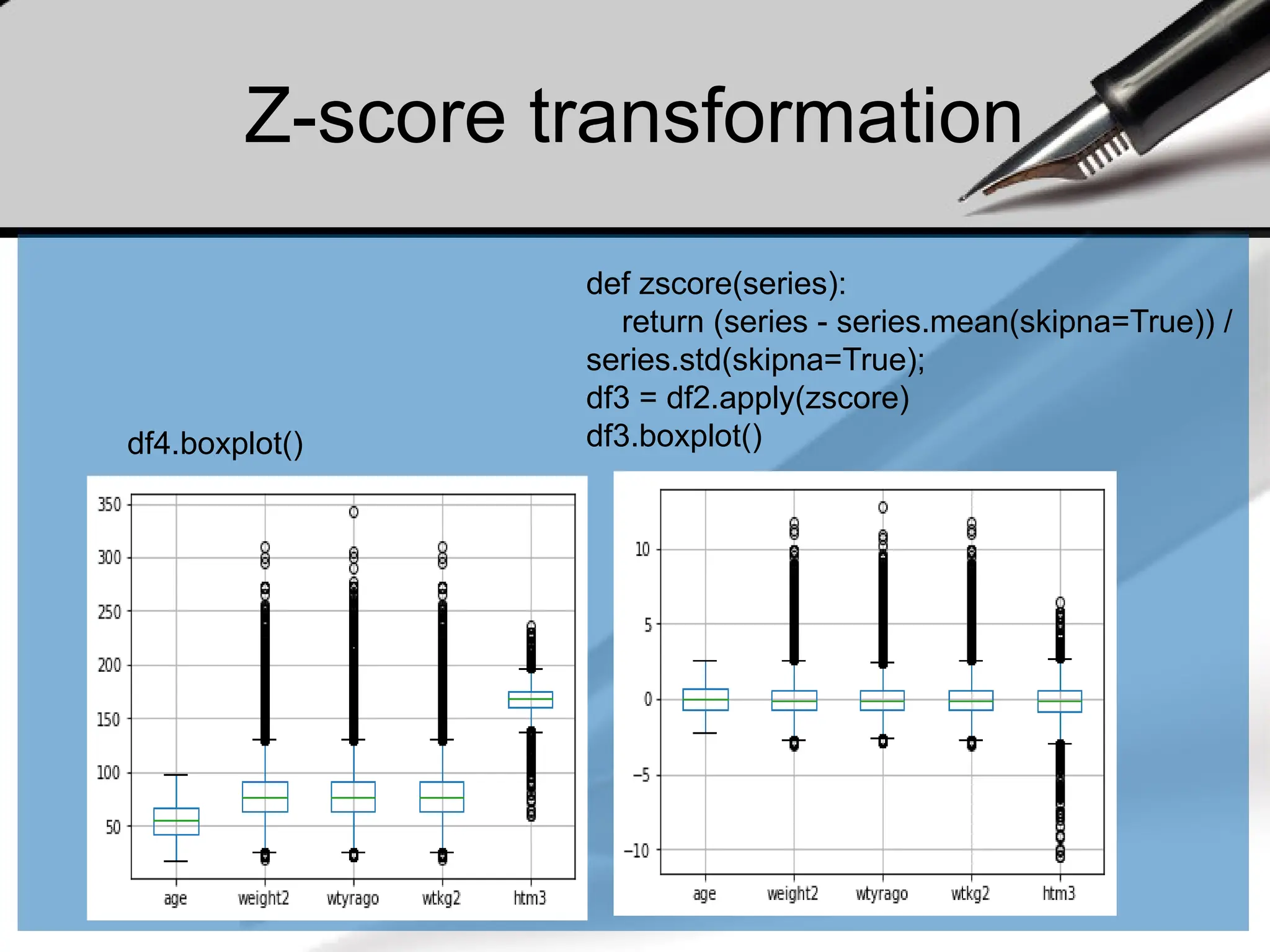
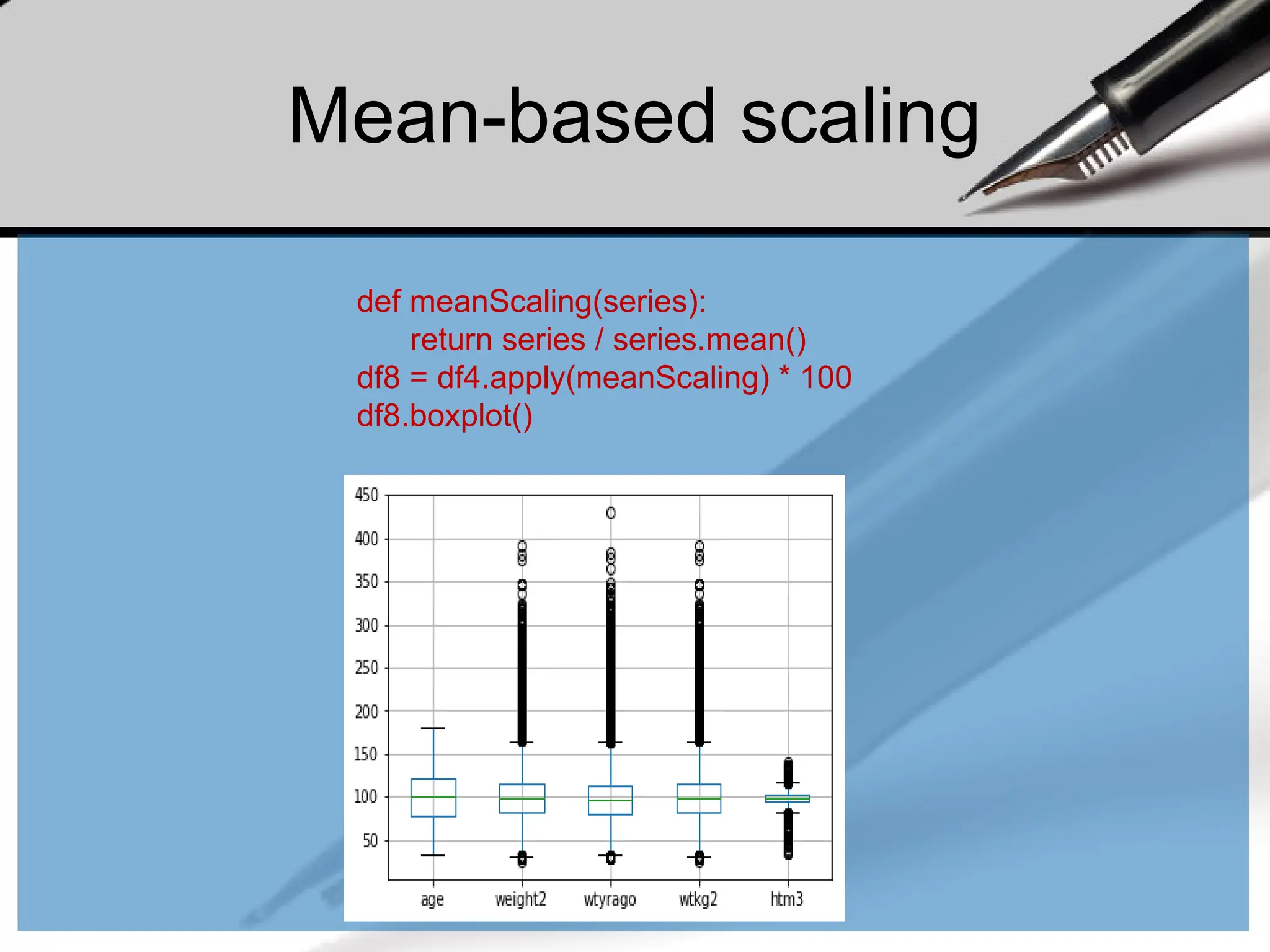

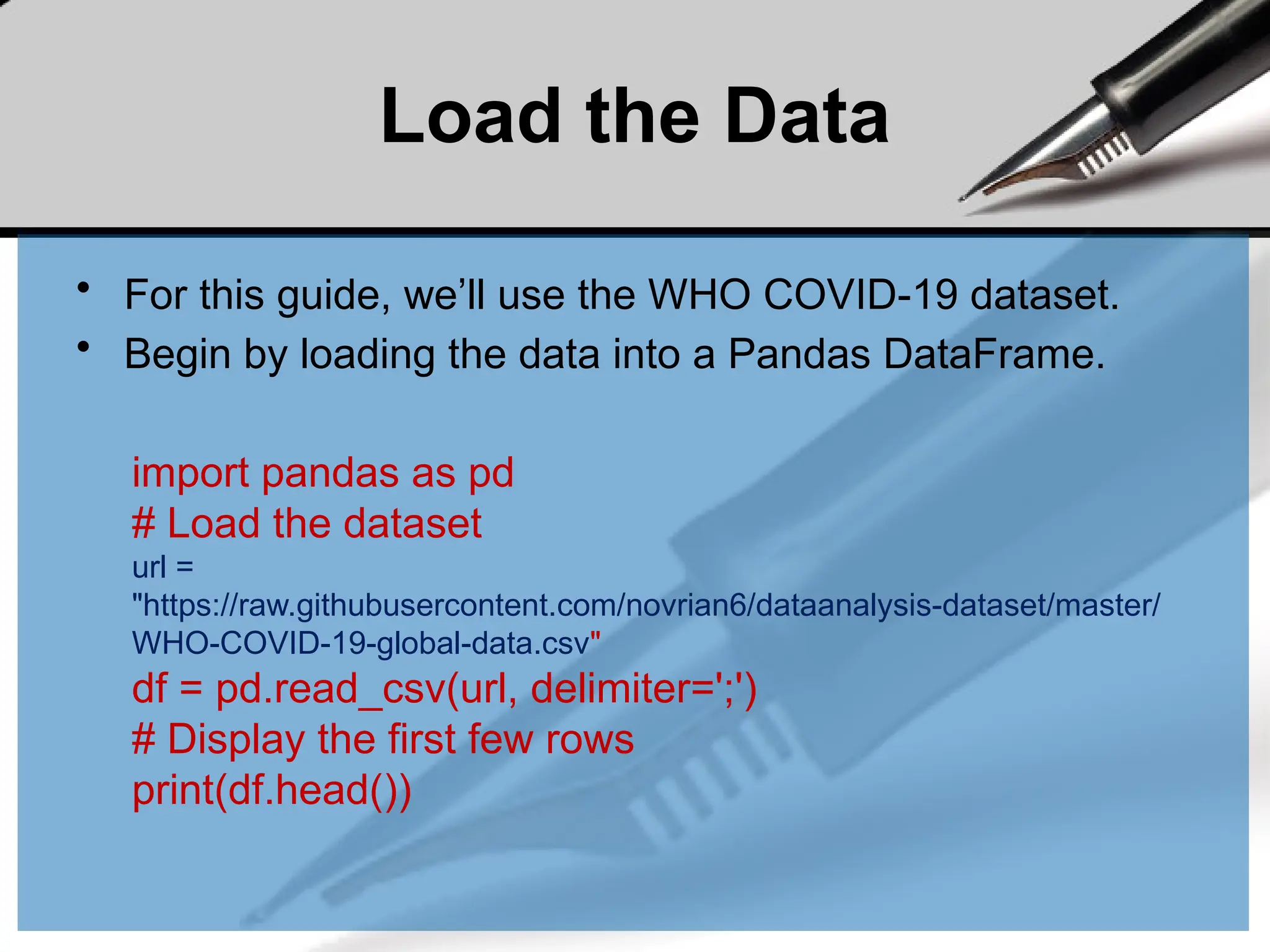
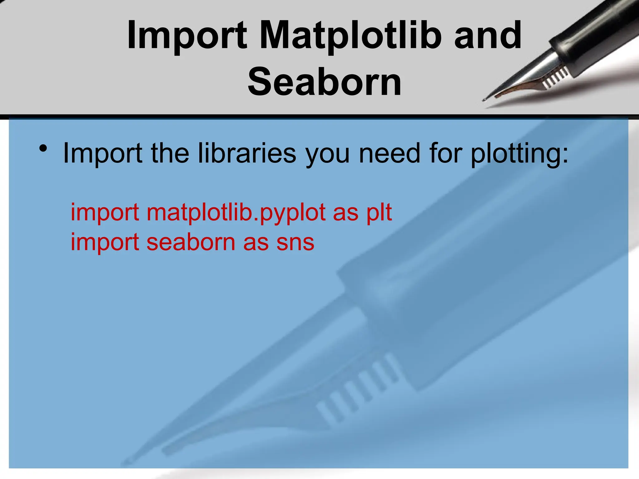
![Basic Plots with Matplotlib
• Matplotlib offers a wide range of plotting functions. Here are
some basic examples:
• Line Plot
• A line plot is useful for visualizing trends over time.
# Convert 'Date_reported' to datetime format
df['Date_reported'] = pd.to_datetime(df['Date_reported'], format='%d/%m/%Y')
# Plot cumulative cases over time for a specific country
df_country = df[df['Country'] == 'Italy']
plt.figure(figsize=(12, 6))
plt.plot(df_country['Date_reported'], df_country['Cumulative_cases'], marker='o', linestyle='-',
color='b', label='Cumulative Cases')
plt.xlabel('Date')
plt.ylabel('Cumulative Cases')
plt.title('Cumulative COVID-19 Cases in Italy')
plt.legend()
plt.grid(True)
plt.show()](https://image.slidesharecdn.com/dalecture1introduction-250915234621-3db310b6/75/DATA-ANALYSIS_Lecture-1-Introduction-pptx-236-2048.jpg)
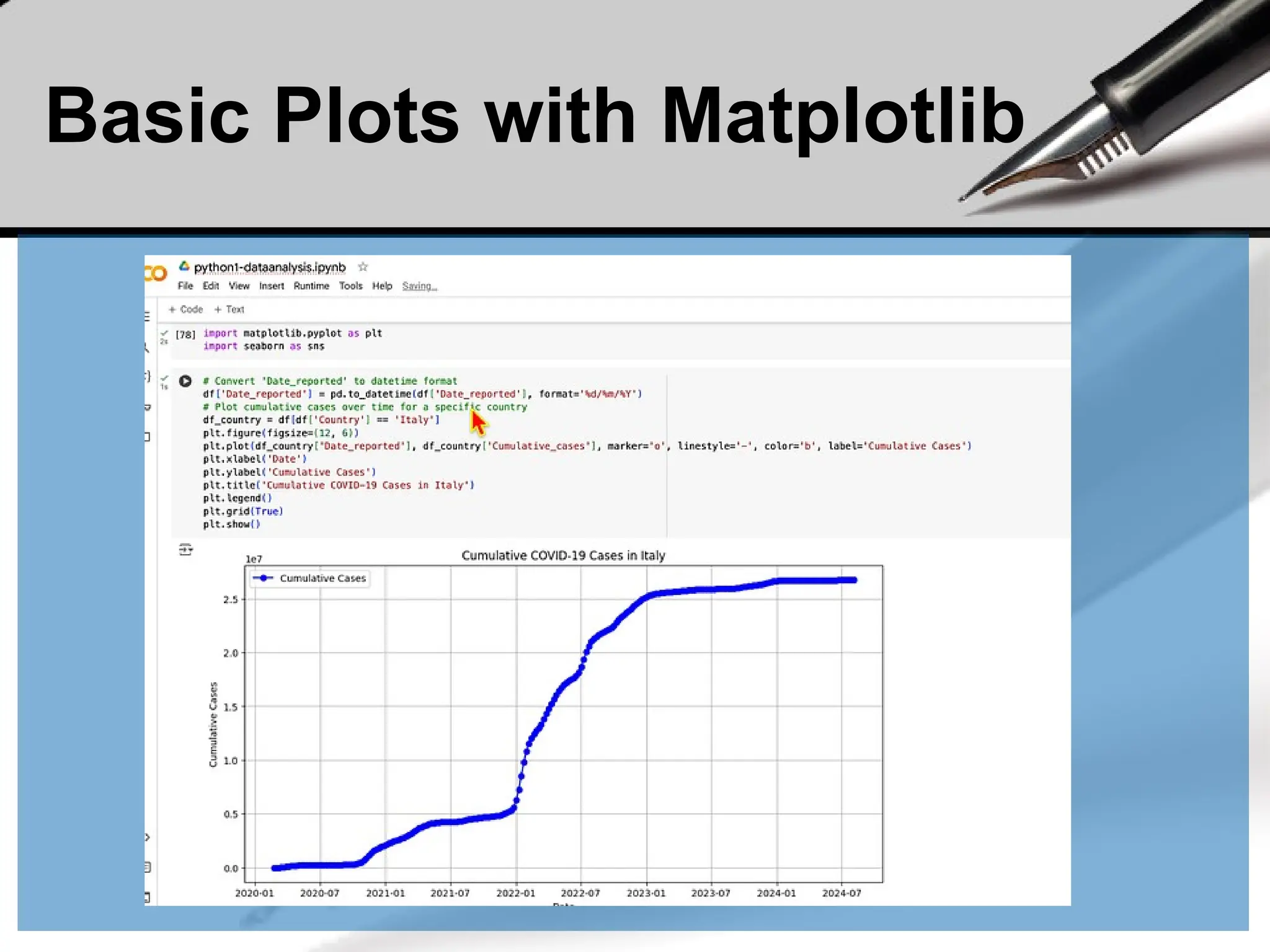
![Basic Plots with Matplotlib
• Bar Plot
• A bar plot is ideal for comparing quantities across different
categories.
# Plot total new cases by country
top_countries = df.groupby('Country')['New_cases'].sum().nlargest(10)
plt.figure(figsize=(14, 8))
top_countries.plot(kind='bar', color='skyblue')
plt.xlabel('Country')
plt.ylabel('New Cases')
plt.title('Top 10 Countries by New COVID-19 Cases')
plt.xticks(rotation=45)
plt.show()](https://image.slidesharecdn.com/dalecture1introduction-250915234621-3db310b6/75/DATA-ANALYSIS_Lecture-1-Introduction-pptx-238-2048.jpg)
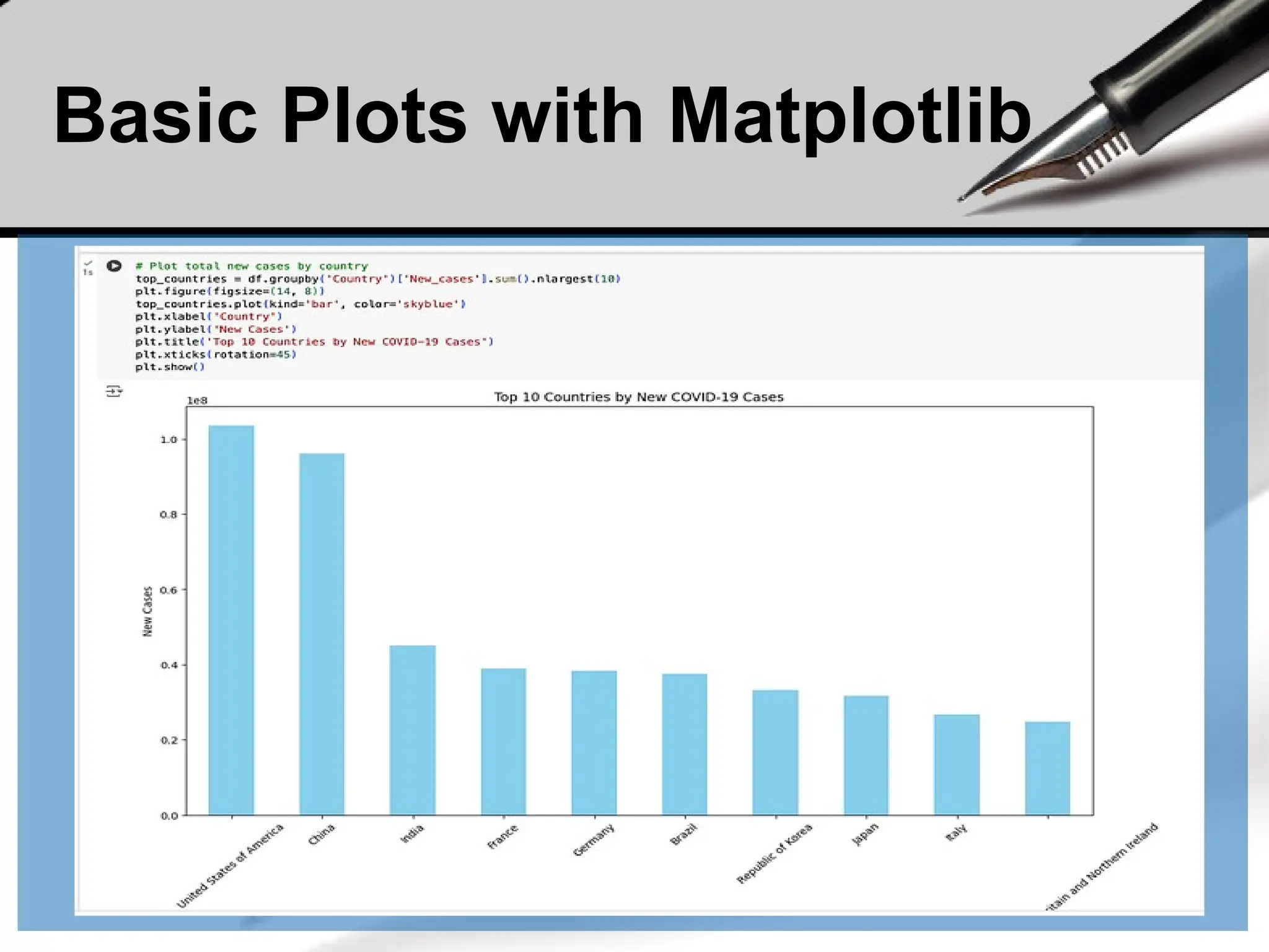
![Basic Plots with Matplotlib
• Histogram
• Histograms show the distribution of a numerical variable.
# Distribution of new cases
plt.figure(figsize=(12, 6))
plt.hist(df['New_cases'], bins=30, color='blue',
edgecolor='black', alpha=0.7)
plt.xlabel('New Cases')
plt.ylabel('Frequency')
plt.title('Distribution of New COVID-19 Cases')
plt.grid(True)
plt.show()](https://image.slidesharecdn.com/dalecture1introduction-250915234621-3db310b6/75/DATA-ANALYSIS_Lecture-1-Introduction-pptx-240-2048.jpg)
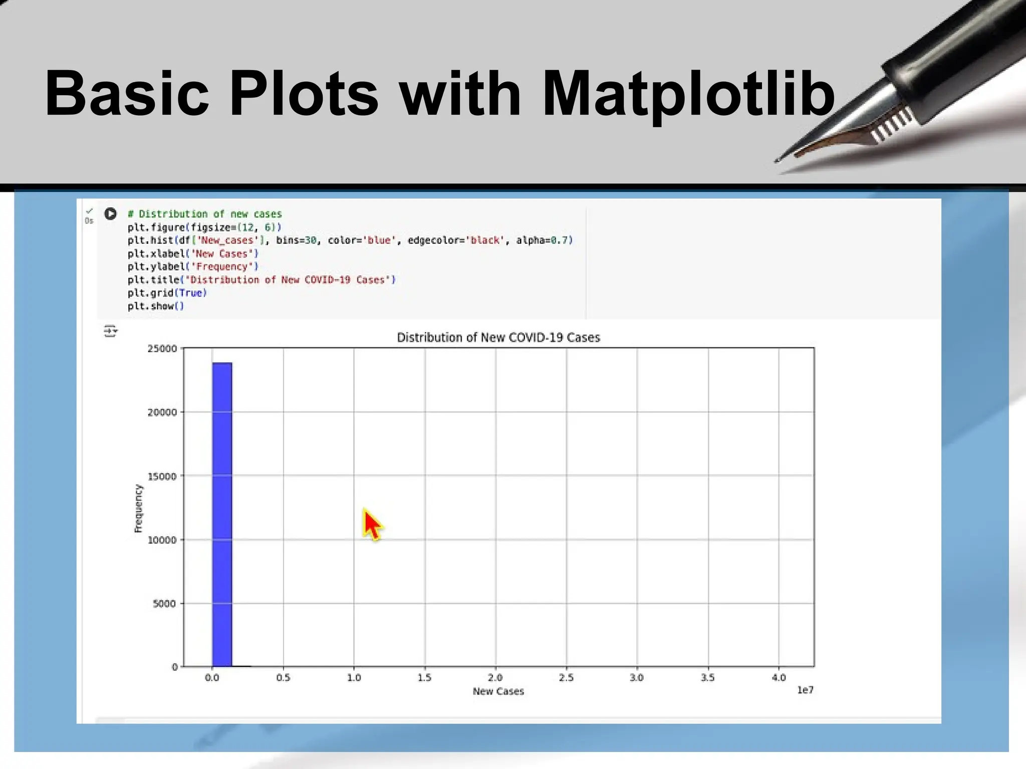
![Basic Plots with Matplotlib
• Scatter Plot
• Scatter plots are used to explore relationships between two
numerical variables.
# Scatter plot of new cases vs. new deaths
plt.figure(figsize=(12, 6))
plt.scatter(df['New_cases'], df['New_deaths'], alpha=0.5,
color='red')
plt.xlabel('New Cases')
plt.ylabel('New Deaths')
plt.title('Scatter Plot of New Cases vs. New Deaths')
plt.grid(True)
plt.show()](https://image.slidesharecdn.com/dalecture1introduction-250915234621-3db310b6/75/DATA-ANALYSIS_Lecture-1-Introduction-pptx-242-2048.jpg)
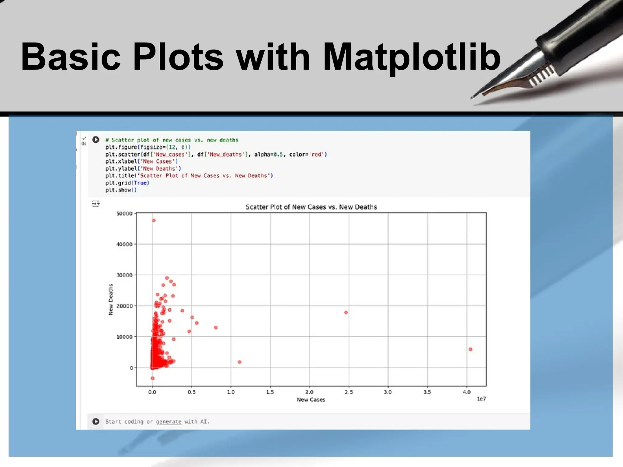
![Advanced Plots with
Seaborn
• Seaborn makes it easy to create aesthetically pleasing
statistical plots.
• Distribution Plot
• A distribution plot visualizes the distribution of a single
variable and can include a Kernel Density Estimate (KDE).
# Distribution of new cases with KDE
plt.figure(figsize=(12, 6))
sns.histplot(df['New_cases'], kde=True, color='blue')
plt.xlabel('New Cases')
plt.ylabel('Frequency')
plt.title('Distribution of New COVID-19 Cases')
plt.show()](https://image.slidesharecdn.com/dalecture1introduction-250915234621-3db310b6/75/DATA-ANALYSIS_Lecture-1-Introduction-pptx-244-2048.jpg)
![Advanced Plots with
Seaborn
• Pair Plot
• A pair plot allows you to visualize relationships between
multiple numerical variables.
# Pair plot of new cases and new deaths
sns.pairplot(df[['New_cases', 'New_deaths']])
plt.show()](https://image.slidesharecdn.com/dalecture1introduction-250915234621-3db310b6/75/DATA-ANALYSIS_Lecture-1-Introduction-pptx-245-2048.jpg)
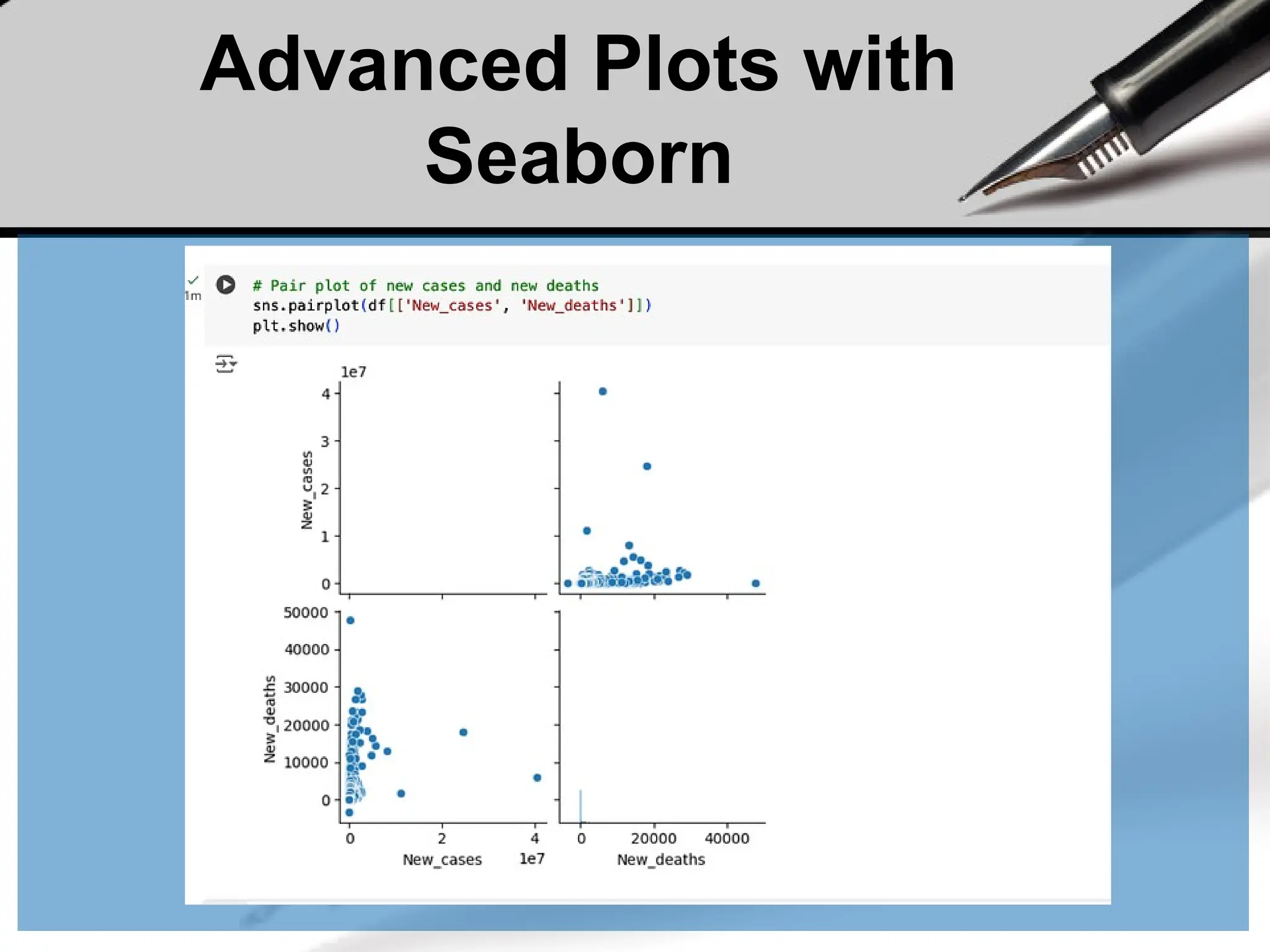
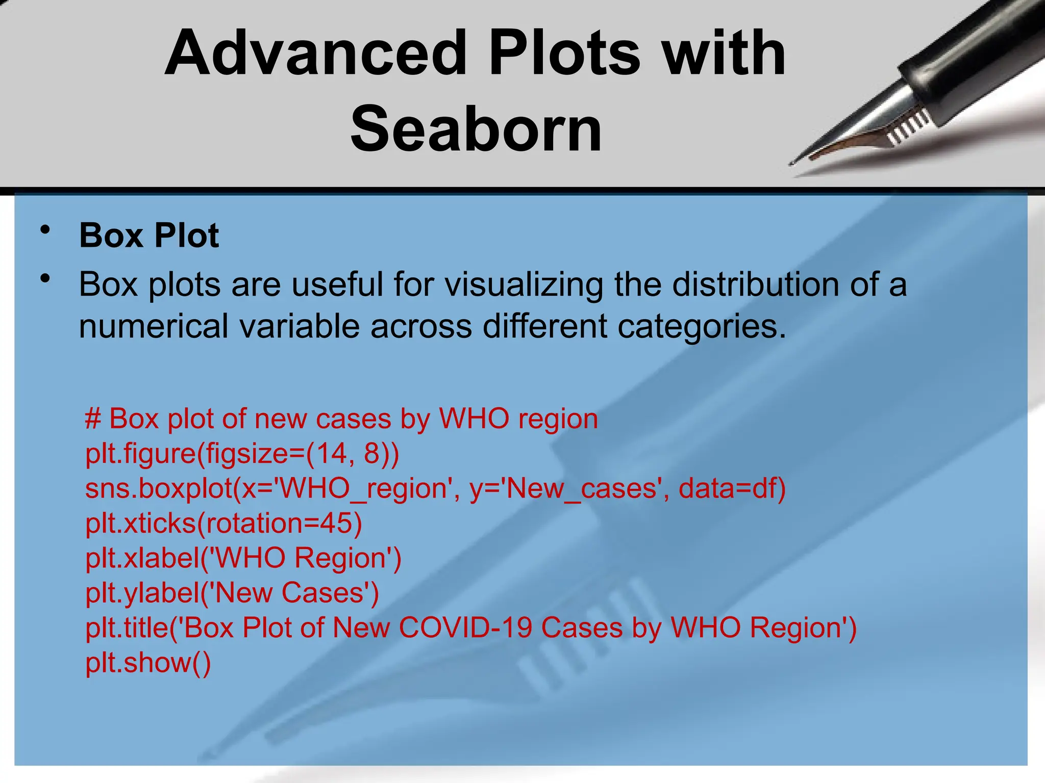
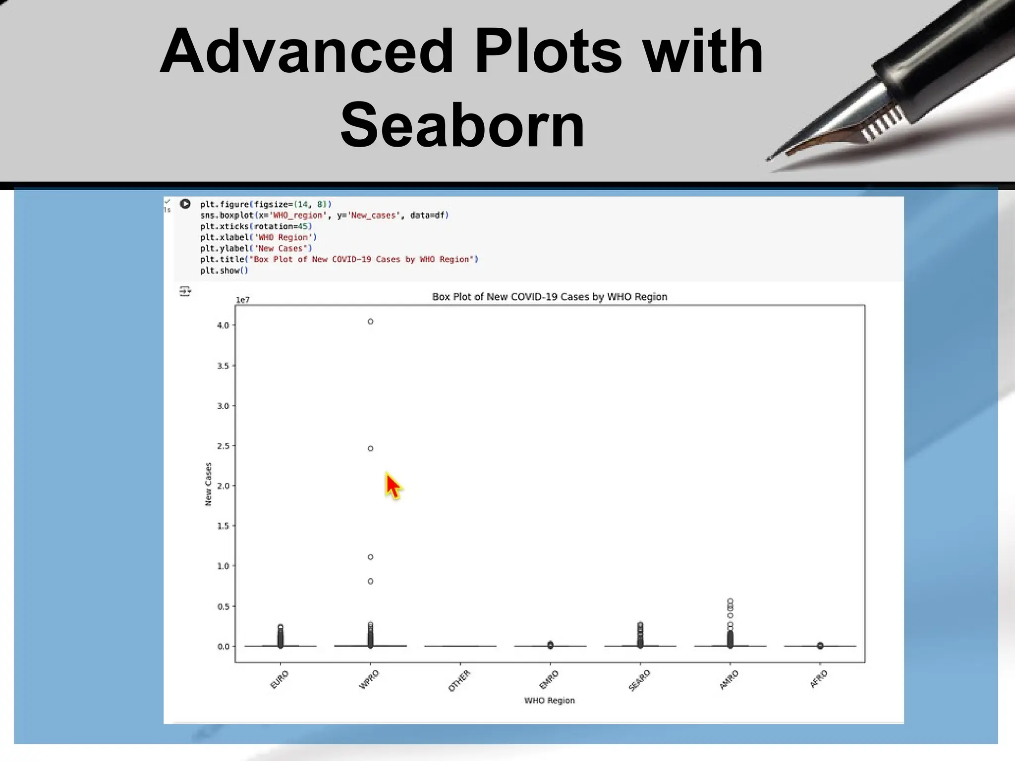
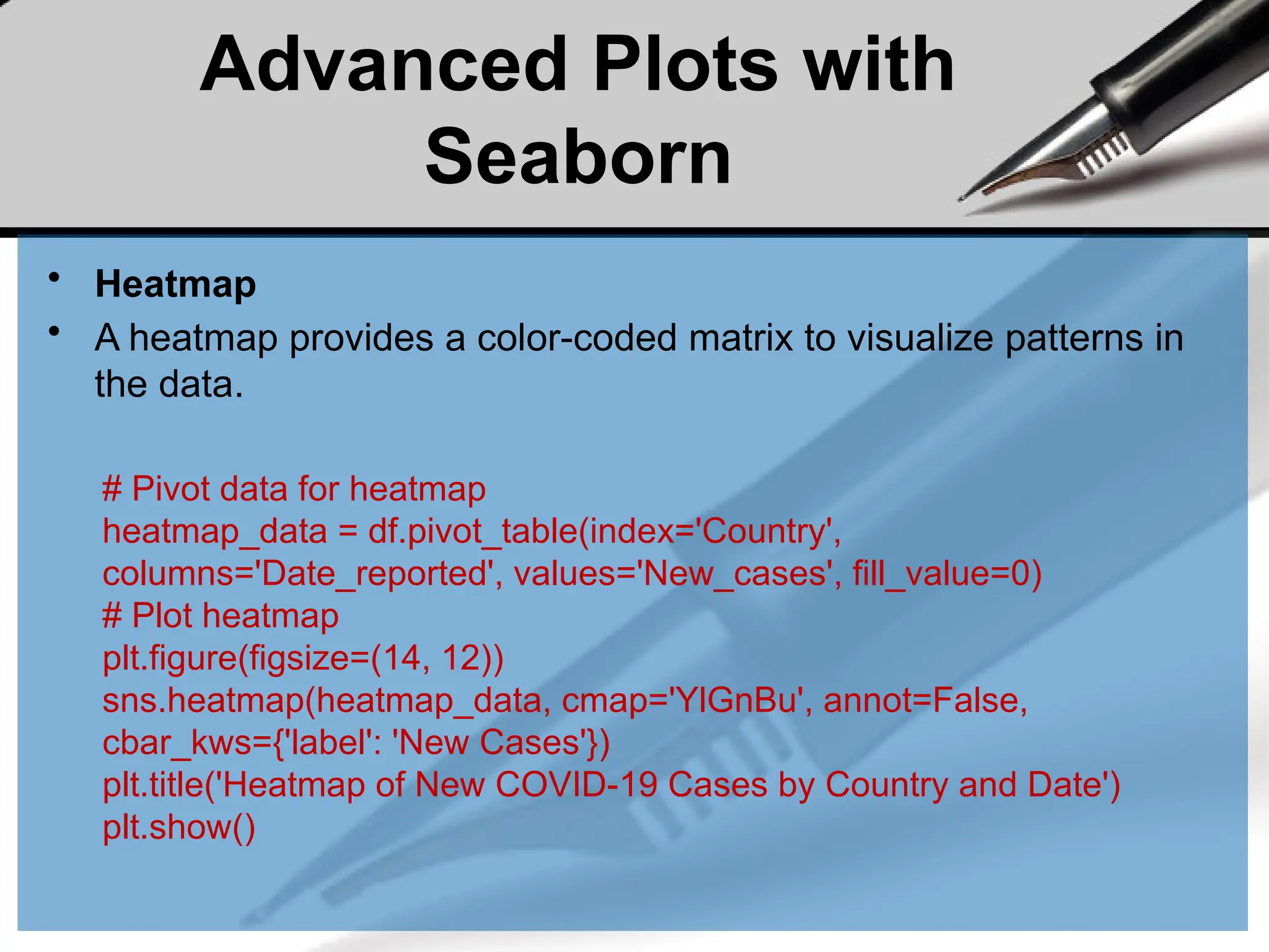
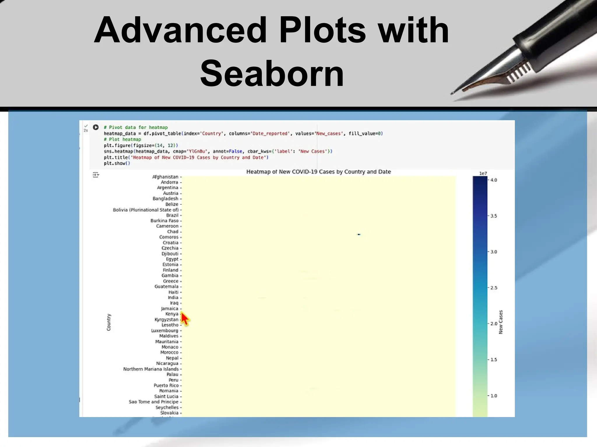
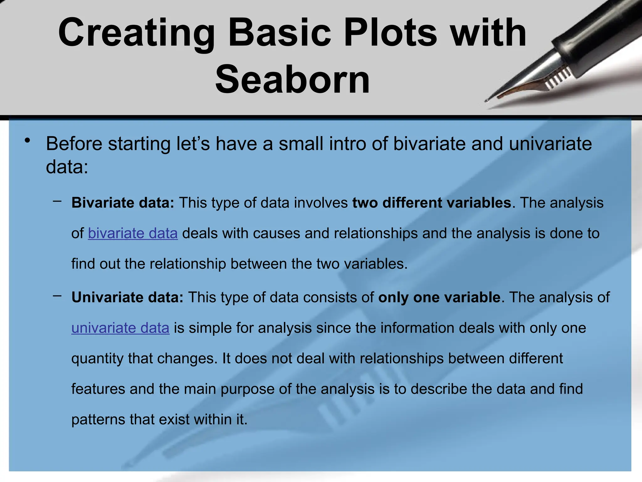
![Creating Basic Plots with
Seaborn
• Lineplot is the most popular plot to draw a relationship
between x and y with the possibility of several semantic
groupings. It is often used to track changes over intervals.
import pandas as pd
import seaborn as sns
data = {'Name':[ 'Mohe' , 'Karnal' , 'Yrik' , 'jack' ],
'Age':[ 30 , 21 , 29 , 28 ]}
df = pd.DataFrame( data )
sns.lineplot( data['Age'], data['Weight'])](https://image.slidesharecdn.com/dalecture1introduction-250915234621-3db310b6/75/DATA-ANALYSIS_Lecture-1-Introduction-pptx-252-2048.jpg)
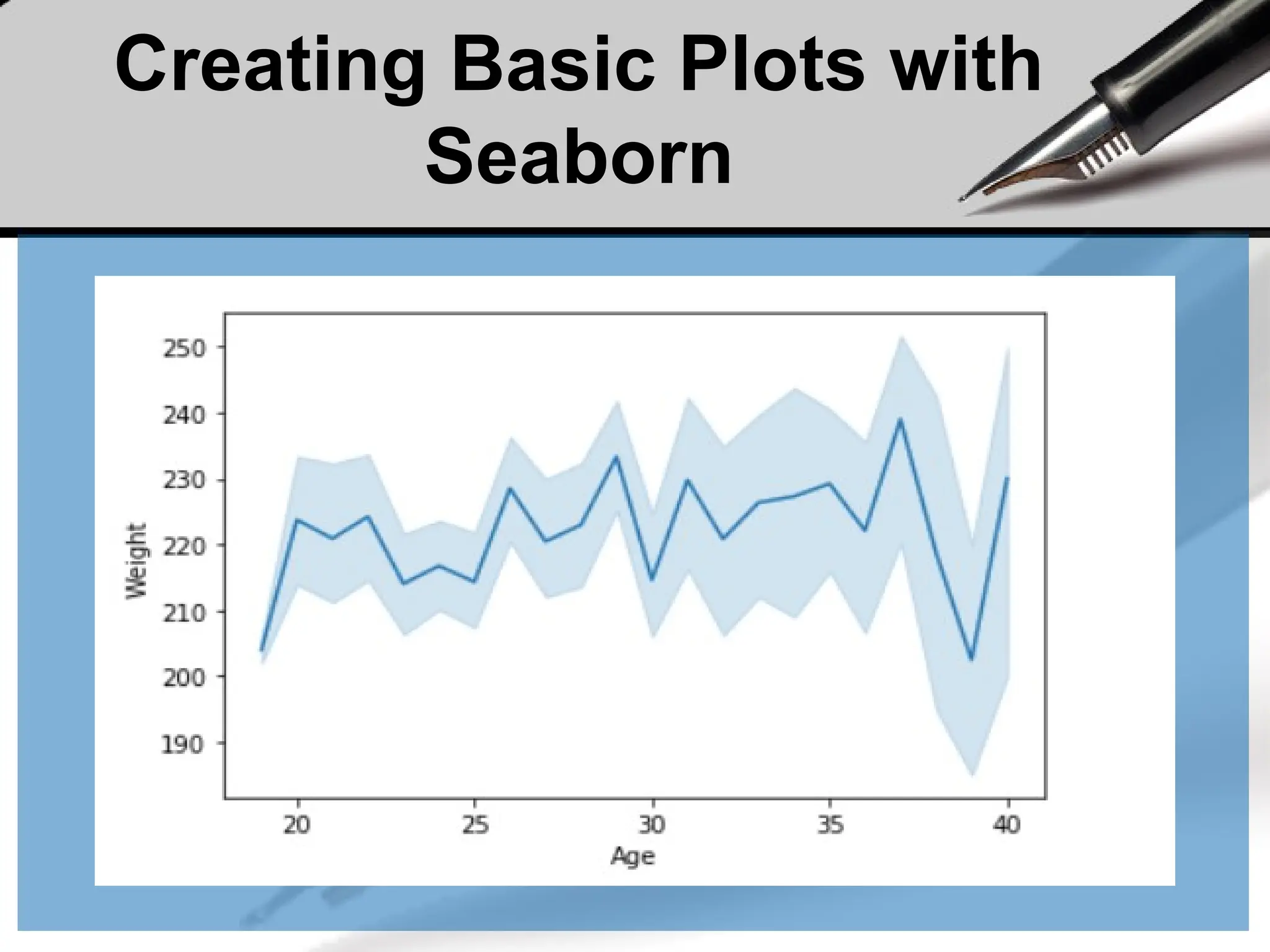
![Creating Basic Plots with
Seaborn
• Scatter plots are used to visualize the relationship between
two numerical variables. They help identify correlations or
patterns. It can draw a two-dimensional graph.
import pandas as pd
import seaborn as sns
data = {'Name':[ 'Mohe' , 'Karnal' , 'Yrik' , 'jack' ], 'Age':[ 30 , 21 , 29 , 28 ]}
df = pd.DataFrame( data )
seaborn.scatterplot(data['Age'],data['Weight'])](https://image.slidesharecdn.com/dalecture1introduction-250915234621-3db310b6/75/DATA-ANALYSIS_Lecture-1-Introduction-pptx-254-2048.jpg)
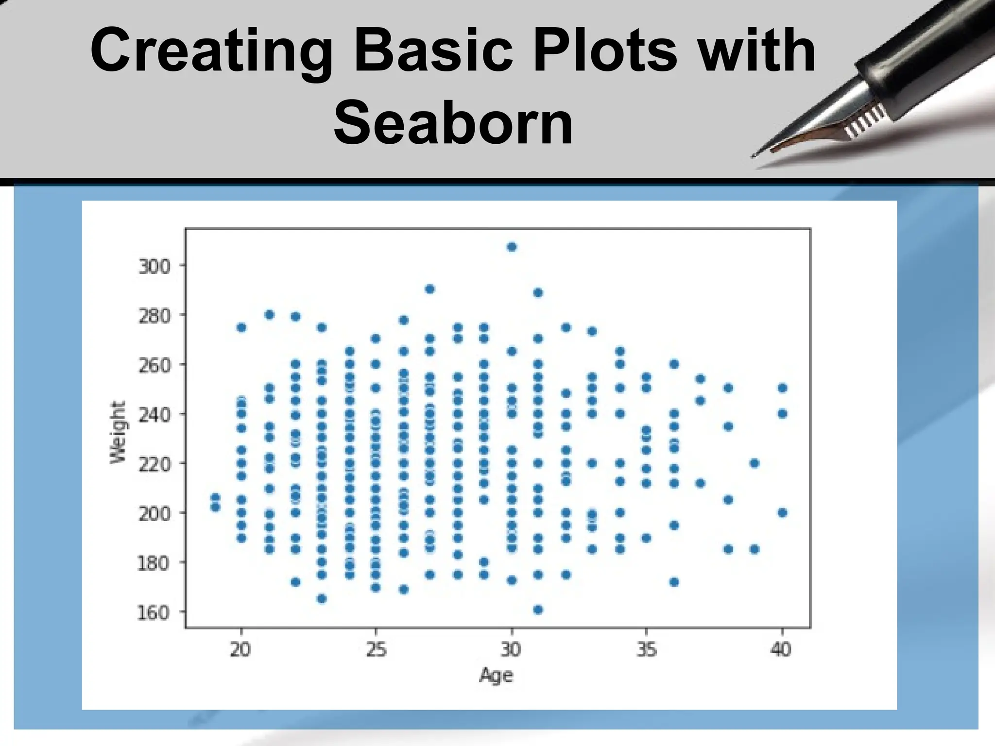
![Creating Basic Plots with
Seaborn
• A box plot is the visual representation of the depicting groups of
numerical data with their quartiles against continuous/categorical data.
• A box plot consists of 5 things Minimum ,First Quartile or 25% , Median
(Second Quartile) or 50%, Third Quartile or 75% and Maximum.
import pandas as pd
import seaborn as sns
# initialise data of lists
data = {'Name':[ 'Mohe' , 'Karnal' , 'Yrik' , 'jack' ], 'Age':[ 30 , 21 , 29 , 28 ]}
df = pd.DataFrame( data )
sns.boxplot( data['Age'] )](https://image.slidesharecdn.com/dalecture1introduction-250915234621-3db310b6/75/DATA-ANALYSIS_Lecture-1-Introduction-pptx-256-2048.jpg)
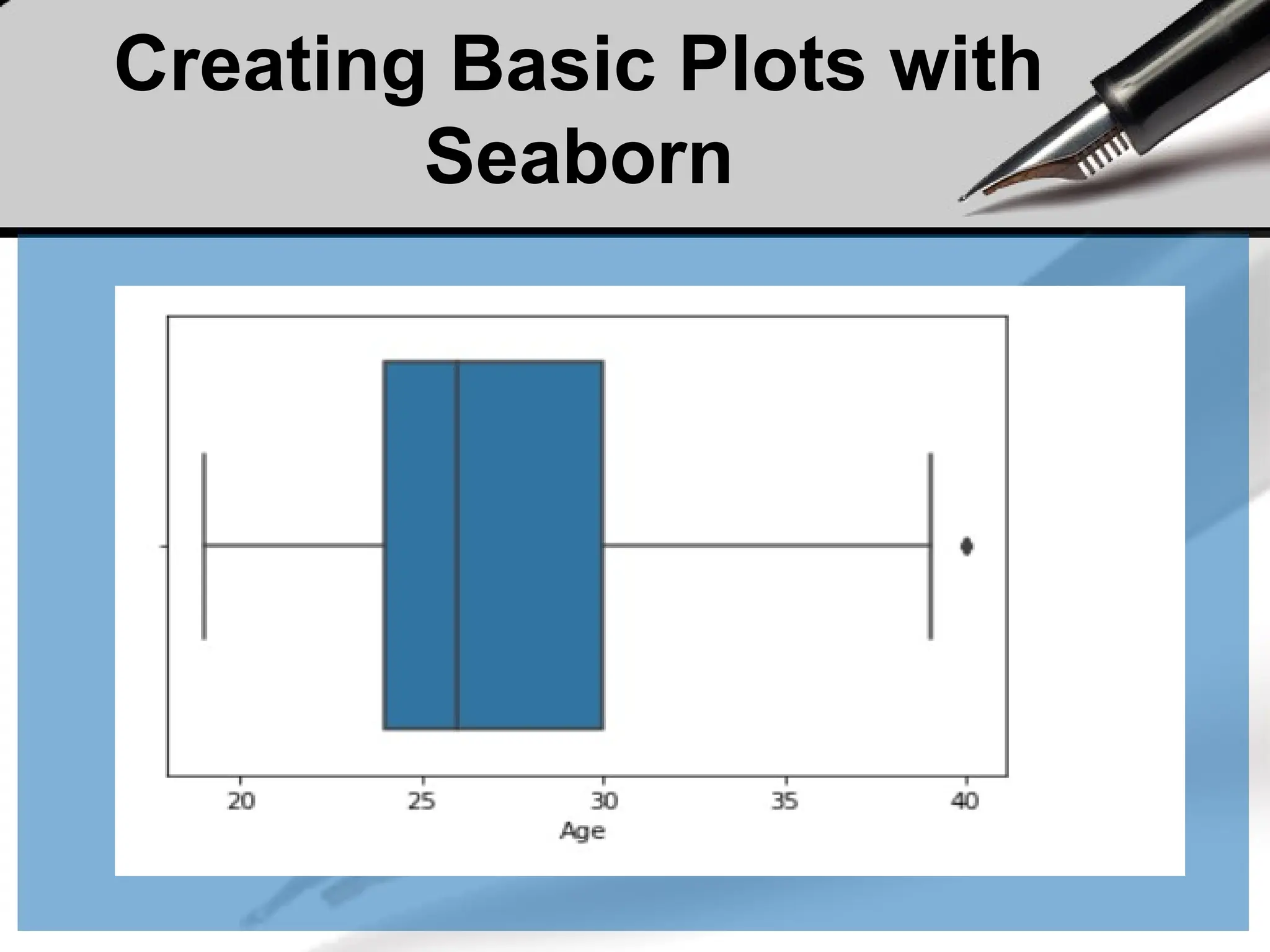
![Creating Basic Plots with
Seaborn
• A violin plot is similar to a boxplot. It shows several
quantitative data across one or more categorical variables
such that those distributions can be compared.
import pandas as pd
import seaborn as sns
# initialise data of lists
data = {'Name':[ 'Mohe' , 'Karnal' , 'Yrik' , 'jack' ], 'Age':[ 30 , 21 , 29 , 28 ]}
df = pd.DataFrame( data )
sns.violinplot(data['Age'])](https://image.slidesharecdn.com/dalecture1introduction-250915234621-3db310b6/75/DATA-ANALYSIS_Lecture-1-Introduction-pptx-258-2048.jpg)
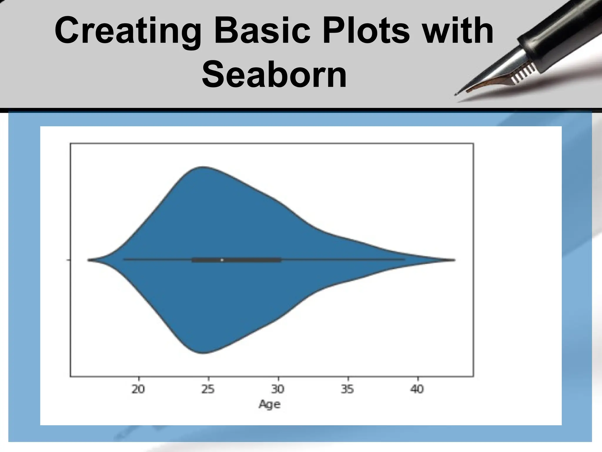
![Creating Basic Plots with
Seaborn
• A swarm plot is similar to a strip plot we can draw a swarm
plot with non-overlapping points against categorical data.
import seaborn
seaborn.set(style = 'whitegrid')
data = pandas.read_csv( "nba.csv" )
seaborn.swarmplot(x = data["Age"])](https://image.slidesharecdn.com/dalecture1introduction-250915234621-3db310b6/75/DATA-ANALYSIS_Lecture-1-Introduction-pptx-260-2048.jpg)
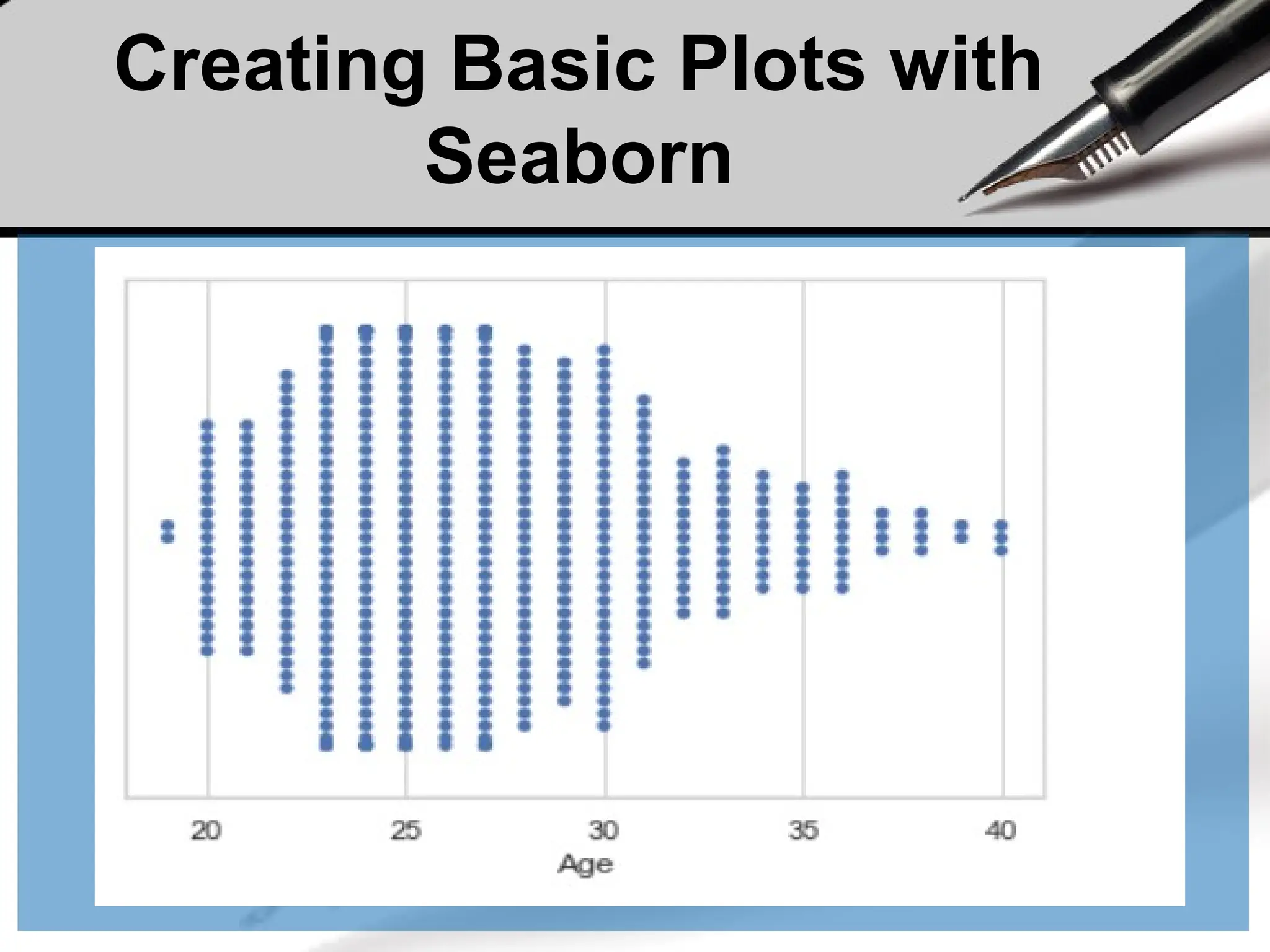
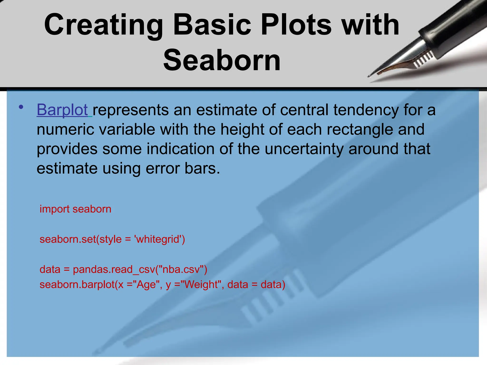
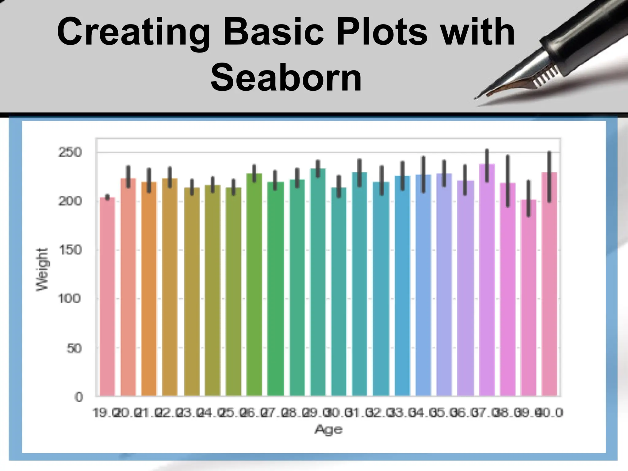
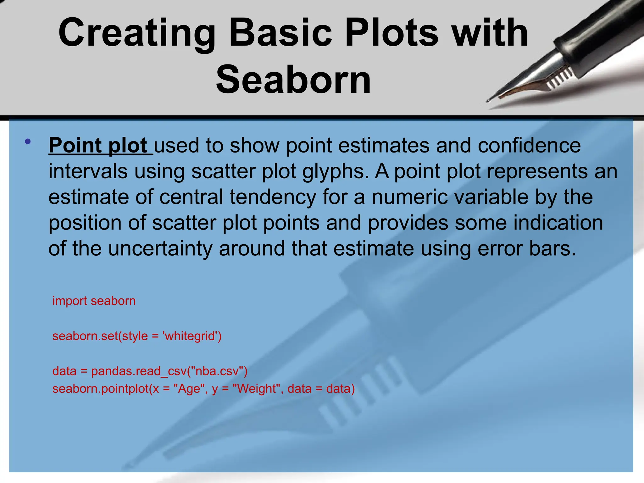
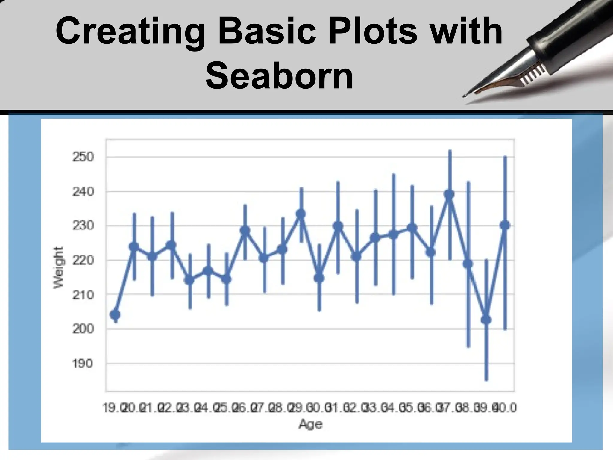
![Creating Basic Plots with
Seaborn
• A Count plot in Seaborn displays the number of occurrences
of each category using bars to visualize the distribution of
categorical variables.
import seaborn
seaborn.set(style = 'whitegrid')
data = pandas.read_csv("nba.csv")
seaborn.countplot(data["Age"])](https://image.slidesharecdn.com/dalecture1introduction-250915234621-3db310b6/75/DATA-ANALYSIS_Lecture-1-Introduction-pptx-266-2048.jpg)
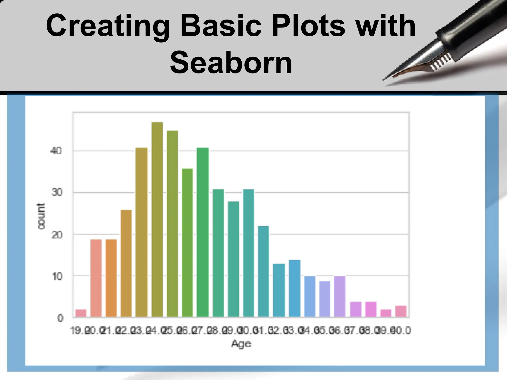
![Creating Basic Plots with
Seaborn
• KDE Plot described as Kernel Density Estimate is used for
visualizing the Probability Density of a continuous variable. It
depicts the probability density at different values in a
continuous variable. We can also plot a single graph for
multiple samples which helps in more efficient data
visualization.
import seaborn as sns
import pandas
data = pandas.read_csv("nba.csv").head()
sns.kdeplot( data['Age'], data['Number'])](https://image.slidesharecdn.com/dalecture1introduction-250915234621-3db310b6/75/DATA-ANALYSIS_Lecture-1-Introduction-pptx-268-2048.jpg)
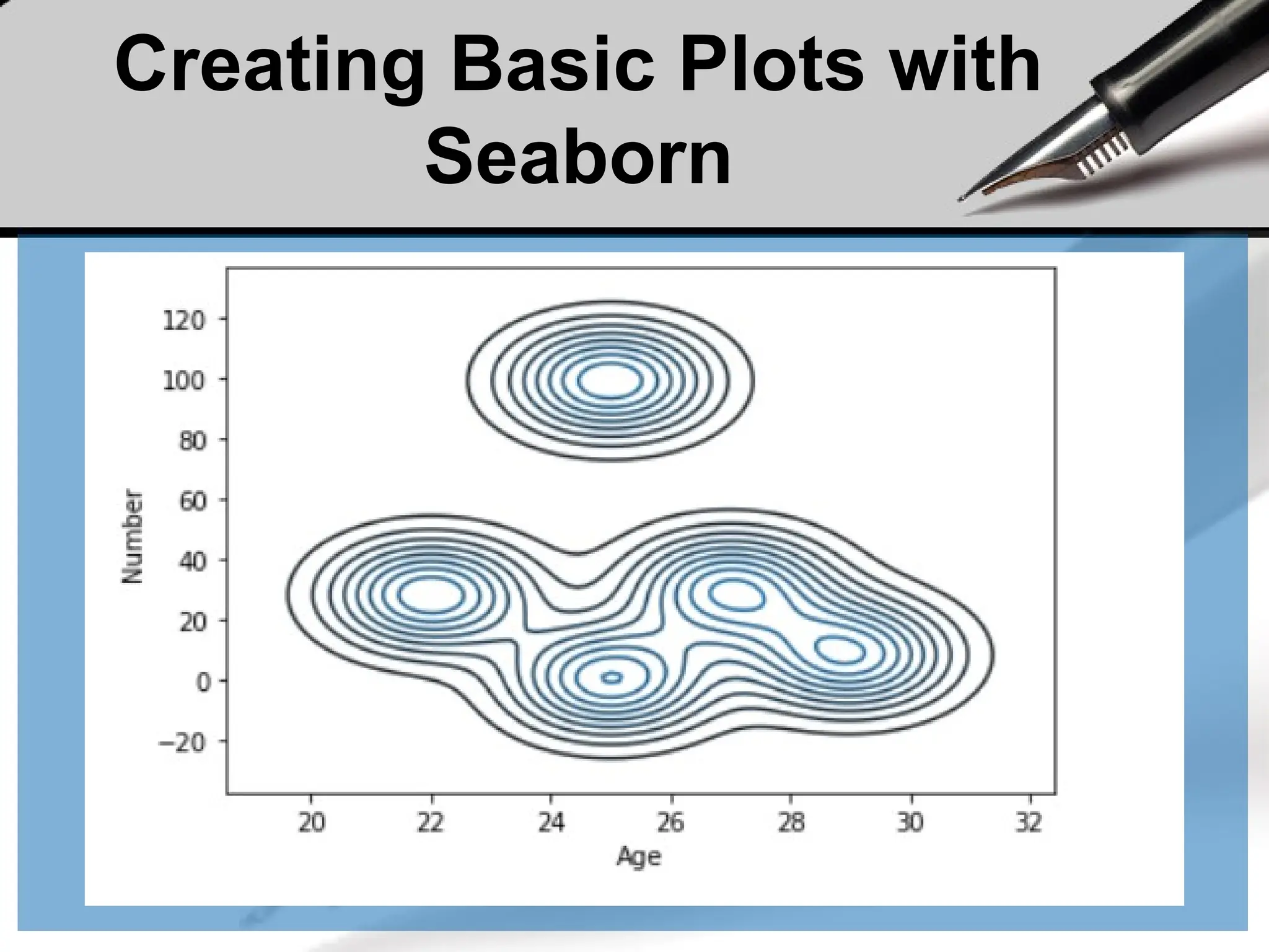
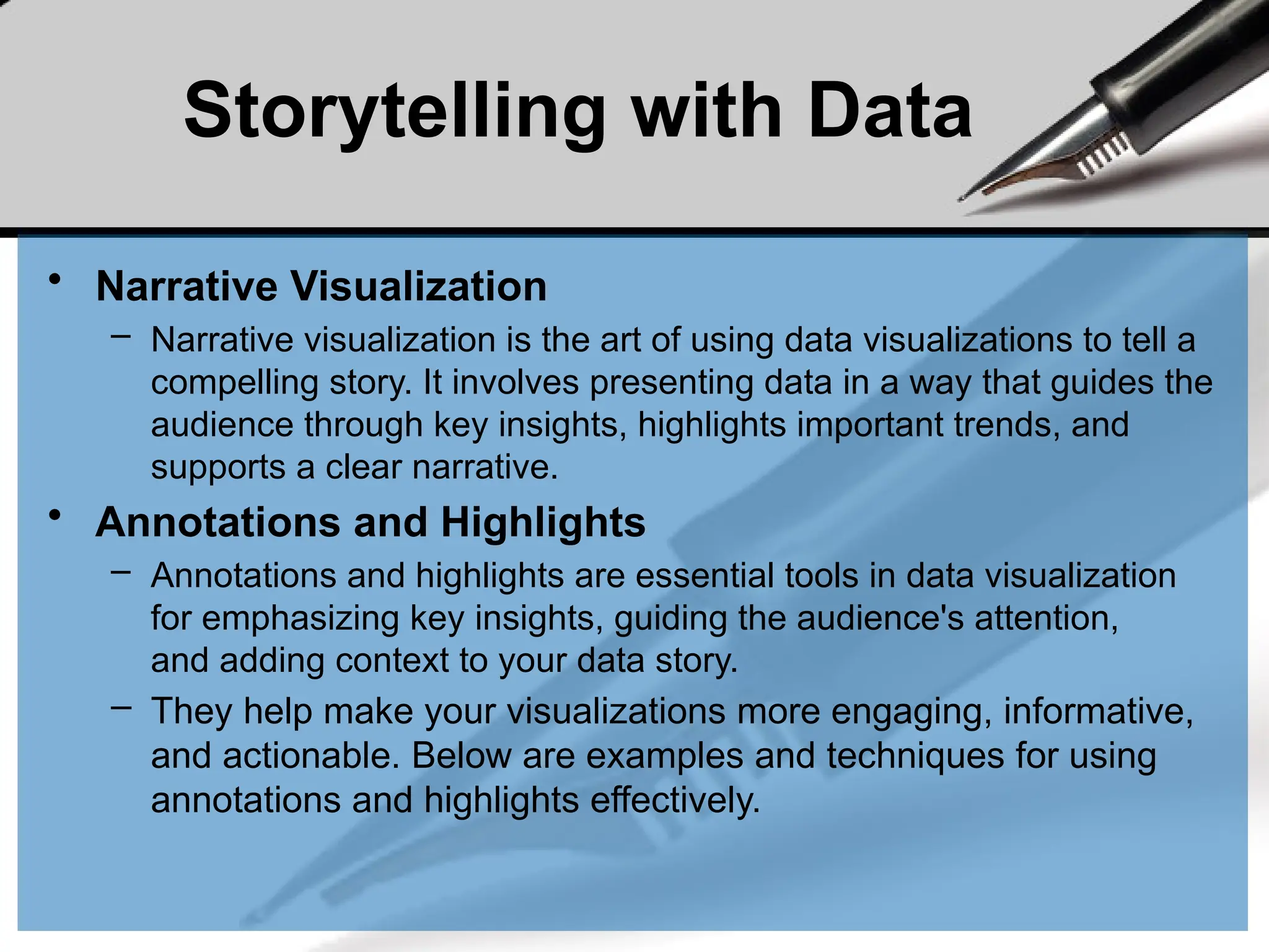


![Demo
• Step-by-Step Analysis
4. Basic Analysis:
Perform some basic analysis to get insights.
# Summary statistics
print(df.describe())
# Total sales and profit per product
total_sales = df.groupby('Product')['Sales'].sum()
total_profit = df.groupby('Product')['Profit'].sum()
print(total_sales)
print(total_profit)](https://crownmelresort.com/image.slidesharecdn.com/dalecture1introduction-250915234621-3db310b6/75/DATA-ANALYSIS_Lecture-1-Introduction-pptx-33-2048.jpg)


![Variable types
• Integer (int)
• Float (float)
• String (str)
• Boolean (bool)
• Complex (complex)
• […]
• User defined
(classes)
• A variable is assigned using the = operator; i.e:
In: Out:
• Create an integer, float, and string
variable.
• Print these to the screen.
• Play around using different variable
names, etc.
• The print() function is used to print
something to the screen.](https://crownmelresort.com/image.slidesharecdn.com/dalecture1introduction-250915234621-3db310b6/75/DATA-ANALYSIS_Lecture-1-Introduction-pptx-46-2048.jpg)


![Lists
• Lists are essentially containers of arbitrary
type.
• They are probably the container that you will
use most frequently.
• The elements of a list can be of different
types.
• The difference between tuples and lists is in
performance; it is much faster to ‘grab’ an
element stored in a tuple, but lists are much
more versatile.
• Note that lists are denoted by [] and not the ()
used by tuples.
In:
Out:
• Create a list and populate it with some elements.](https://crownmelresort.com/image.slidesharecdn.com/dalecture1introduction-250915234621-3db310b6/75/DATA-ANALYSIS_Lecture-1-Introduction-pptx-58-2048.jpg)


![The range() function
• The range() function generates a list of numbers, which is generally used to
iterate over within for loops.
• The range() function has two sets of parameters to follow:
range(stop)
stop: Number of integers
(whole numbers) to generate,
starting from zero. i.e:
range([start], stop[, step])
start: Starting number of the sequence.
stop: Generate numbers up to, but not including this
number.
step: Difference between each number in the
sequence. i.e.:
Note:
• All parameters must be integers.
• Parameters can be positive or negative.
• The range() function (and Python in general) is 0-index based, meaning list indexes start at 0,
not 1. eg. The syntax to access the first element of a list is mylist[0]. Therefore the last
integer generated by range() is up to, but not including, stop.](https://crownmelresort.com/image.slidesharecdn.com/dalecture1introduction-250915234621-3db310b6/75/DATA-ANALYSIS_Lecture-1-Introduction-pptx-67-2048.jpg)


![Our first plot
• You may be wondering why the x-axis ranges
from 0-3 and the y-axis from 1-4.
• If you provide a single list or array to the plot()
command, Matplotlib assumes it is a
sequence of y values, and automatically
generates the x values for you.
• Since python ranges start with 0, the default
x vector has the same length as y but starts
with 0.
• Hence the x data are [0,1,2,3].](https://crownmelresort.com/image.slidesharecdn.com/dalecture1introduction-250915234621-3db310b6/75/DATA-ANALYSIS_Lecture-1-Introduction-pptx-96-2048.jpg)


![The axis() function
• The axis() function allows us to specify the range of the axis.
• It requires a list that contains the following:
[The min x-axis value, the max x-axis value, the min y-axis, the max y-axis value]](https://crownmelresort.com/image.slidesharecdn.com/dalecture1introduction-250915234621-3db310b6/75/DATA-ANALYSIS_Lecture-1-Introduction-pptx-103-2048.jpg)


![ndarray
• ndarray is used for storage of homogeneous data
– i.e., all elements the same type
• Every array must have a shape and a dtype
• Supports convenient slicing, indexing and efficient
vectorized computation
import numpy as np
data1 = [6, 7.5, 8, 0, 1]
arr1 = np.array(data1)
print(arr1)
print(arr1.dtype)
print(arr1.shape)
print(arr1.ndim)
[6. 7.5 8. 0. 1. ]
float64
(5,)
1](https://crownmelresort.com/image.slidesharecdn.com/dalecture1introduction-250915234621-3db310b6/75/DATA-ANALYSIS_Lecture-1-Introduction-pptx-126-2048.jpg)
![Creating ndarrays
Using list of lists
import numpy as np
data2 = [[1, 2, 3, 4], [5, 6, 7, 8]] #list of lists
arr2 = np.array(data2)
print(arr2.ndim) #2
print(arr2.shape) # (2,4)](https://crownmelresort.com/image.slidesharecdn.com/dalecture1introduction-250915234621-3db310b6/75/DATA-ANALYSIS_Lecture-1-Introduction-pptx-127-2048.jpg)
![array = np.array([[0,1,2],[2,3,4]])
[[0 1 2]
[2 3 4]]
array = np.zeros((2,3))
[[0. 0. 0.]
[0. 0. 0.]]
array = np.ones((2,3))
[[1. 1. 1.]
[1. 1. 1.]]
array = np.eye(3)
[[1. 0. 0.]
[0. 1. 0.]
[0. 0. 1.]]
array = np.arange(0, 10, 2)
[0, 2, 4, 6, 8]
array = np.random.randint(0,
10, (3,3))
[[6 4 3]
[1 5 6]
[9 8 5]]
Creating ndarrays
arange is an array-valued version of the built-in Python range function](https://crownmelresort.com/image.slidesharecdn.com/dalecture1introduction-250915234621-3db310b6/75/DATA-ANALYSIS_Lecture-1-Introduction-pptx-128-2048.jpg)
![Arithmatic with NumPy Arrays
• Any arithmetic operations between equal-size
arrays applies the operation element-wise:
arr = np.array([[1., 2., 3.], [4., 5., 6.]])
print(arr)
[[1. 2. 3.]
[4. 5. 6.]]
print(arr * arr)
[[ 1. 4. 9.]
[16. 25. 36.]]
print(arr - arr)
[[0. 0. 0.]
[0. 0. 0.]]](https://crownmelresort.com/image.slidesharecdn.com/dalecture1introduction-250915234621-3db310b6/75/DATA-ANALYSIS_Lecture-1-Introduction-pptx-129-2048.jpg)
![Arithmatic with NumPy Arrays
• Arithmetic operations with scalars propagate the scalar argument to
each element in the array:
• Comparisons between arrays of the same size yield boolean arrays:
arr = np.array([[1., 2., 3.], [4., 5., 6.]])
print(arr)
[[1. 2. 3.]
[4. 5. 6.]]
print(arr **2)
[[ 1. 4. 9.]
[16. 25. 36.]]
arr2 = np.array([[0., 4., 1.], [7., 2., 12.]])
print(arr2)
[[ 0. 4. 1.]
[ 7. 2. 12.]]
print(arr2 > arr)
[[False True False]
[ True False True]]](https://crownmelresort.com/image.slidesharecdn.com/dalecture1introduction-250915234621-3db310b6/75/DATA-ANALYSIS_Lecture-1-Introduction-pptx-130-2048.jpg)
![Indexing and Slicing
• One-dimensional arrays are simple; on the
surface they act similarly to Python lists:
arr = np.arange(10)
print(arr) # [0 1 2 3 4 5 6 7 8 9]
print(arr[5]) #5
print(arr[5:8]) #[5 6 7]
arr[5:8] = 12
print(arr) #[ 0 1 2 3 4 12 12 12 8 9]](https://crownmelresort.com/image.slidesharecdn.com/dalecture1introduction-250915234621-3db310b6/75/DATA-ANALYSIS_Lecture-1-Introduction-pptx-131-2048.jpg)
![Indexing and Slicing
• As you can see, if you assign a scalar value to a slice, as in arr[5:8] =
12, the value is propagated (or broadcasted) to the entire selection.
• An important first distinction from Python’s built-in lists is that array
slices are views on the original array.
– This means that the data is not copied, and any modifications to the view
will be reflected in the source array.
arr = np.arange(10)
print(arr) # [0 1 2 3 4 5 6 7 8 9]
arr_slice = arr[5:8]
print(arr_slice) # [5 6 7]
arr_slice[1] = 12345
print(arr) # [ 0 1 2 3 4 5 12345 7 8 9]
arr_slice[:] = 64
print(arr) # [ 0 1 2 3 4 64 64 64 8 9]](https://crownmelresort.com/image.slidesharecdn.com/dalecture1introduction-250915234621-3db310b6/75/DATA-ANALYSIS_Lecture-1-Introduction-pptx-132-2048.jpg)
![Indexing
• In a two-dimensional array, the elements at each index are
no longer scalars but rather one-dimensional arrays:
• Thus, individual elements can be accessed recursively.
But that is a bit too much work, so you can pass a comma-
separated list of indices to select individual elements.
• So these are equivalent:
arr2d = np.array([[1, 2, 3], [4, 5, 6], [7, 8, 9]])
print(arr2d[2]) # [7 8 9]
print(arr2d[0][2]) # 3
print(arr2d[0, 2]) #3](https://crownmelresort.com/image.slidesharecdn.com/dalecture1introduction-250915234621-3db310b6/75/DATA-ANALYSIS_Lecture-1-Introduction-pptx-133-2048.jpg)
![Activity
• Consider the two-dimensional array, arr2d.
• Write a code to slice this array to display the last
column,
[[3] [6] [9]]
• Write a code to slice this array to display the last
2 elements of middle array,
[5 6]
arr2d = np.array([[1, 2, 3], [4, 5, 6], [7, 8, 9]])](https://crownmelresort.com/image.slidesharecdn.com/dalecture1introduction-250915234621-3db310b6/75/DATA-ANALYSIS_Lecture-1-Introduction-pptx-134-2048.jpg)


![Series
• One dimensional array-like object
• It contains array of data (of any NumPy data type) with
associated indexes. (Indexes can be strings or integers
or other data types.)
• By default , the series will get indexing from 0 to N where
N = size -1
from pandas import Series, DataFrame
import pandas as pd
obj = Series([4, 7, -5, 3])
print(obj)
print(obj.index)
print(obj.values)
#Output
0 4
1 7
2 -5
3 3
dtype: int64
RangeIndex(start=0, stop=4, step=1)
[ 4 7 -5 3]](https://crownmelresort.com/image.slidesharecdn.com/dalecture1introduction-250915234621-3db310b6/75/DATA-ANALYSIS_Lecture-1-Introduction-pptx-138-2048.jpg)
![Series – referencing elements
obj2 = Series([4, 7, -5, 3], index=['d', 'b', 'a', 'c'])
print(obj2)
#Output
d 4
b 7
a -5
c 3
dtype: int64
print(obj2.index)
#Output
Index(['d', 'b', 'a', 'c'], dtype='object')
print(obj2.values)
#Output
[ 4 7 -5 3]
print(obj2['a'])
#Output
-5
obj2['d']= 10
print(obj2[['d', 'c', 'a']])
#Output
d 10
c 3
a -5
dtype: int64
print(obj2[:2])
#Output
d 10
b 7
dtype: int64
print(obj2.a)
#Output
-5](https://crownmelresort.com/image.slidesharecdn.com/dalecture1introduction-250915234621-3db310b6/75/DATA-ANALYSIS_Lecture-1-Introduction-pptx-139-2048.jpg)
![Series – array/dict operations
numpy array operations can also be applied,
which will preserve the index-value link
obj4 = obj3[obj3>0]
print(obj4)
#output
d 10
b 7
c 3
dtype: int64
print(obj3**2)
#output
d 100
b 49
a 25
c 9
dtype: int64
print(‘b’ in obj3)
#output
true
Can be thought of as a dict.
Can be constructed from a dict directly.
obj3 = Series({'d': 4, 'b': 7, 'a': -5, 'c':3 })
print(obj3)
#output
d 4
b 7
a -5
c 3
dtype: int64](https://crownmelresort.com/image.slidesharecdn.com/dalecture1introduction-250915234621-3db310b6/75/DATA-ANALYSIS_Lecture-1-Introduction-pptx-140-2048.jpg)
![Series – from dictionary
sdata = {'Texas': 10, 'Ohio': 20, 'Oregon': 15, 'Utah': 18}
states = ['Texas', 'Ohio', 'Oregon', 'Iowa']
obj4 = Series(sdata, index=states)
print(obj4)
#output
Texas 10.0
Ohio 20.0
Oregon 15.0
Iowa NaN
dtype: float64
Missing value
print(pd.isnull(obj4))
#output
Texas False
Ohio False
Oregon False
Iowa True
dtype: bool
print(pd.notnull(obj4))
#output
Texas True
Ohio True
Oregon True
Iowa False
dtype: bool
print(obj4[obj4.notnull()])
#output
Texas 10.0
Ohio 20.0
Oregon 15.0
dtype: float64
dictionary](https://crownmelresort.com/image.slidesharecdn.com/dalecture1introduction-250915234621-3db310b6/75/DATA-ANALYSIS_Lecture-1-Introduction-pptx-141-2048.jpg)
![Series – auto alignment
print(obj4.add(obj5))
#output
Iowa NaN
Ohio 40.0
Oregon 30.0
Texas 20.0
Utah NaN
dtype: float64
sdata = {'Texas': 10, 'Ohio': 20, 'Oregon': 15, 'Utah': 18}
states = ['Texas', 'Ohio', 'Oregon', 'Iowa']
obj4 = Series(sdata, index=states)
print(obj4)
#Output
Texas 10.0
Ohio 20.0
Oregon 15.0
Iowa NaN
dtype: float64
sdata = {'Texas': 10, 'Ohio': 20, 'Oregon': 15, 'Utah': 18}
states = ['Texas', 'Ohio', 'Oregon', 'Utah']
obj5 = Series(sdata, index=states)
print(obj5)
#Output
Texas 10
Ohio 20
Oregon 15
Utah 18
dtype: int64](https://crownmelresort.com/image.slidesharecdn.com/dalecture1introduction-250915234621-3db310b6/75/DATA-ANALYSIS_Lecture-1-Introduction-pptx-142-2048.jpg)
![Series name and index name
sdata = {'Texas': 10, 'Ohio': 20, 'Oregon': 15, 'Utah': 18}
states = ['Texas', 'Ohio', 'Oregon', 'Iowa']
obj4 = Series(sdata, index=states)
obj4.name = 'population'
obj4.index.name = 'state'
print(obj4)
#output
state
Texas 10.0
Ohio 20.0
Oregon 15.0
Iowa NaN
Name: population, dtype: float64](https://crownmelresort.com/image.slidesharecdn.com/dalecture1introduction-250915234621-3db310b6/75/DATA-ANALYSIS_Lecture-1-Introduction-pptx-143-2048.jpg)
![Series name and index name
• Index of a series can be changed to a different index.
obj4.index = ['Florida', 'New York', 'Kentucky', 'Georgia']
Florida 10.0
New York 20.0
Kentucky 15.0
Georgia NaN
Name: population, dtype: float64
• Index object itself is immutable.
obj4.index[2]='California'
TypeError: Index does not support mutable operations
print(obj4.index)
Index(['Florida', 'New York', 'Kentucky', 'Georgia'], dtype='object')](https://crownmelresort.com/image.slidesharecdn.com/dalecture1introduction-250915234621-3db310b6/75/DATA-ANALYSIS_Lecture-1-Introduction-pptx-144-2048.jpg)
![Indexing, selection and filtering
• Series can be sliced/accessed with label-based
indexes, or using position-based indexes
S = Series(range(4), index=['zero', 'one', 'two', 'three'])
print(S['two'])
2
print(S[['zero', 'two']])
zero 0
two 2
dtype: int64
print(S[2])
2
print(S[[0,2]])
zero 0
two 2
dtype: int64
list operator for items >1](https://crownmelresort.com/image.slidesharecdn.com/dalecture1introduction-250915234621-3db310b6/75/DATA-ANALYSIS_Lecture-1-Introduction-pptx-145-2048.jpg)
![Indexing, selection and filtering
• Series can be sliced/accessed with label-based
indexes, or using position-based indexes
S = Series(range(4), index=['zero', 'one', 'two', 'three'])
print(S[:2])
zero 0
one 1
dtype: int32
print(S['zero': 'two'])
zero 0
one 1
two 2
dtype: int32
Inclusive
print(S[S > 1])
two 2
three 3
dtype: int32
print(S[-2:])
two 2
three 3
dtype: int32](https://crownmelresort.com/image.slidesharecdn.com/dalecture1introduction-250915234621-3db310b6/75/DATA-ANALYSIS_Lecture-1-Introduction-pptx-146-2048.jpg)

![DataFrame
• A DataFrame is a tabular data structure comprised of rows and
columns, akin to a spreadsheet or database table.
• It can be treated as an ordered collection of columns
– Each column can be a different data type
– Have both row and column indices
data = {'state': ['Ohio', 'Ohio', 'Ohio', 'Nevada', 'Nevada'],
'year': [2000, 2001, 2002, 2001, 2002],
'pop': [1.5, 1.7, 3.6, 2.4, 2.9]}
frame = DataFrame(data)
print(frame)
#output
state year pop
0 Ohio 2000 1.5
1 Ohio 2001 1.7
2 Ohio 2002 3.6
3 Nevada 2001 2.4
4 Nevada 2002 2.9](https://crownmelresort.com/image.slidesharecdn.com/dalecture1introduction-250915234621-3db310b6/75/DATA-ANALYSIS_Lecture-1-Introduction-pptx-148-2048.jpg)
![DataFrame – specifying
columns and indices
• Order of columns/rows can be specified.
• Columns not in data will have NaN.
frame2 = DataFrame(data, columns=['year', 'state', 'pop', 'debt'], index=['A', 'B', 'C', 'D', 'E'])
Print(frame2)
year state pop debt
A 2000 Ohio 1.5 NaN
B 2001 Ohio 1.7 NaN
C 2002 Ohio 3.6 NaN
D 2001 Nevada 2.4 NaN
E 2002 Nevada 2.9 NaN
Same order
Initialized with NaN](https://crownmelresort.com/image.slidesharecdn.com/dalecture1introduction-250915234621-3db310b6/75/DATA-ANALYSIS_Lecture-1-Introduction-pptx-149-2048.jpg)

![DataFrame – index, columns,
values
frame3.index.name = 'year'
frame3.columns.name='state‘
print(frame3)
state Nevada Ohio
year
2000 NaN 1.5
2001 2.9 1.7
2002 2.9 3.6
print(frame3.index)
Int64Index([2000, 2001, 2002], dtype='int64', name='year')
print(frame3.columns)
Index(['Nevada', 'Ohio'], dtype='object', name='state')
print(frame3.values)
[[nan 1.5]
[2.9 1.7]
[2.9 3.6]]](https://crownmelresort.com/image.slidesharecdn.com/dalecture1introduction-250915234621-3db310b6/75/DATA-ANALYSIS_Lecture-1-Introduction-pptx-151-2048.jpg)
![DataFrame – retrieving a
column
• A column in a DataFrame can be retrieved as a Series
by dict-like notation or as attribute
data = {'state': ['Ohio', 'Ohio', 'Ohio', 'Nevada', 'Nevada'],
'year': [2000, 2001, 2002, 2001, 2002],
'pop': [1.5, 1.7, 3.6, 2.4, 2.9]}
frame = DataFrame(data)
print(frame['state'])
0 Ohio
1 Ohio
2 Ohio
3 Nevada
4 Nevada
Name: state, dtype: object
print(frame.state)
0 Ohio
1 Ohio
2 Ohio
3 Nevada
4 Nevada
Name: state, dtype: object](https://crownmelresort.com/image.slidesharecdn.com/dalecture1introduction-250915234621-3db310b6/75/DATA-ANALYSIS_Lecture-1-Introduction-pptx-152-2048.jpg)

![DataFrame – getting rows
• loc for using indexes and iloc for using positions
– loc gets rows (or columns) with particular labels from the index.
– iloc gets rows (or columns) at particular positions in the index (so it only takes integers).
data = {'state': ['Ohio', 'Ohio', 'Ohio', 'Nevada', 'Nevada'],
'year': [2000, 2001, 2002, 2001, 2002],
'pop': [1.5, 1.7, 3.6, 2.4, 2.9]}
frame2 = DataFrame(data, columns=['year', 'state', 'pop', 'debt'], index=['A', 'B', 'C', 'D', 'E'])
print(frame2)
year state pop debt
A 2000 Ohio 1.5 NaN
B 2001 Ohio 1.7 NaN
C 2002 Ohio 3.6 NaN
D 2001 Nevada 2.4 NaN
E 2002 Nevada 2.9 NaN
print(frame2.loc['A'])
year 2000
state Ohio
pop 1.5
debt NaN
Name: A, dtype: object
print(frame2.loc[['A', 'B']])
year state pop debt
A 2000 Ohio 1.5 NaN
B 2001 Ohio 1.7 NaN
print(frame2.loc['A':'E',
['state','pop']])
state pop
A Ohio 1.5
B Ohio 1.7
C Ohio 3.6
D Nevada 2.4
E Nevada 2.9
print(frame2.iloc[1:3])
year state pop debt
B 2001 Ohio 1.7 NaN
C 2002 Ohio 3.6 NaN
print(frame2.iloc[:,1:3])
state pop
A Ohio 1.5
B Ohio 1.7
C Ohio 3.6
D Nevada 2.4
E Nevada 2.9](https://crownmelresort.com/image.slidesharecdn.com/dalecture1introduction-250915234621-3db310b6/75/DATA-ANALYSIS_Lecture-1-Introduction-pptx-154-2048.jpg)
![DataFrame – modifying
columns
frame2['debt'] = 0
print(frame2)
year state pop debt
A 2000 Ohio 1.5 0
B 2001 Ohio 1.7 0
C 2002 Ohio 3.6 0
D 2001 Nevada 2.4 0
E 2002 Nevada 2.9 0
frame2['debt'] = range(5)
print(frame2)
year state pop debt
A 2000 Ohio 1.5 0
B 2001 Ohio 1.7 1
C 2002 Ohio 3.6 2
D 2001 Nevada 2.4 3
E 2002 Nevada 2.9 4
val = Series([10, 10, 10], index = ['A', 'C', 'D'])
frame2['debt'] = val
print(frame2)
year state pop debt
A 2000 Ohio 1.5 10.0
B 2001 Ohio 1.7 NaN
C 2002 Ohio 3.6 10.0
D 2001 Nevada 2.4 10.0
E 2002 Nevada 2.9 NaN
Rows or individual elements can be
modified similarly. Using loc or iloc.](https://crownmelresort.com/image.slidesharecdn.com/dalecture1introduction-250915234621-3db310b6/75/DATA-ANALYSIS_Lecture-1-Introduction-pptx-155-2048.jpg)
![DataFrame:removing columns
del frame2['debt']
print(frame2)
year state pop
A 2000 Ohio 1.5
B 2001 Ohio 1.7
C 2002 Ohio 3.6
D 2001 Nevada 2.4
E 2002 Nevada 2.9](https://crownmelresort.com/image.slidesharecdn.com/dalecture1introduction-250915234621-3db310b6/75/DATA-ANALYSIS_Lecture-1-Introduction-pptx-156-2048.jpg)
![More on DataFrame indexing
import numpy as np
data = np.arange(9).reshape(3,3)
print(data)
[[0 1 2]
[3 4 5]
[6 7 8]]
frame = DataFrame(data, index=['r1', 'r2', 'r3'], columns=['c1', 'c2', 'c3'])
print(frame)
c1 c2 c3
r1 0 1 2
r2 3 4 5
r3 6 7 8
print(frame['c1'])
r1 0
r2 3
r3 6
Name: c1, dtype: int32
print(frame['c1']['r1'])
0
print(frame[['c1', 'c3']])
c1 c3
r1 0 2
r2 3 5
r3 6 8
print(frame.loc['r1'])
c1 0
c2 1
c3 2
Name: r1, dtype: int32
print(frame.loc[['r1','r3']])
c1 c2 c3
r1 0 1 2
r3 6 7 8
print(frame[:2])
c1 c2 c3
r1 0 1 2
r2 3 4 5
print(frame.iloc[:2])
c1 c2 c3
r1 0 1 2
r2 3 4 5
Row slices](https://crownmelresort.com/image.slidesharecdn.com/dalecture1introduction-250915234621-3db310b6/75/DATA-ANALYSIS_Lecture-1-Introduction-pptx-157-2048.jpg)
![More on DataFrame indexing
print(frame.loc[['r1', 'r2'], ['c1', 'c2']])
c1 c2
r1 0 1
r2 3 4
print(frame.iloc[:2,:2])
c1 c2
r1 0 1
r2 3 4
v = DataFrame(np.arange(9).reshape(3,3), index=['a', 'a', 'b'], columns=['c1','c2','c3'])
print(v)
c1 c2 c3
a 0 1 2
a 3 4 5
b 6 7 8
print(v.loc['a'])
c1 c2 c3
a 0 1 2
a 3 4 5
Duplicated keys
print(frame.loc['r1':'r3', 'c1':'c3'])
c1 c2 c3
r1 0 1 2
r2 3 4 5
r3 6 7 8](https://crownmelresort.com/image.slidesharecdn.com/dalecture1introduction-250915234621-3db310b6/75/DATA-ANALYSIS_Lecture-1-Introduction-pptx-158-2048.jpg)
![More on DataFrame indexing
print(frame)
c1 c2 c3
r1 0 1 2
r2 3 4 5
r3 6 7 8
print(frame <3)
c1 c2 c3
r1 True True True
r2 False False False
r3 False False False
print(frame[frame['c1']>0])
c1 c2 c3
r2 3 4 5
r3 6 7 8
print(frame['c1']>0)
r1 False
r2 True
r3 True
Name: c1, dtype: bool
frame[frame<3] = 3
print(frame)
c1 c2 c3
r1 3 3 3
r2 3 4 5
r3 6 7 8](https://crownmelresort.com/image.slidesharecdn.com/dalecture1introduction-250915234621-3db310b6/75/DATA-ANALYSIS_Lecture-1-Introduction-pptx-159-2048.jpg)

![Removing rows/columns
print(frame)
c1 c2 c3
r1 0 1 2
r2 3 4 5
r3 6 7 8
print(frame.drop(['r1']))
c1 c2 c3
r2 3 4 5
r3 6 7 8
print(frame.drop(['r1','r3']))
c1 c2 c3
r2 3 4 5
print(frame.drop(['c1'], axis=1))
c2 c3
r1 1 2
r2 4 5
r3 7 8
This returns a new object](https://crownmelresort.com/image.slidesharecdn.com/dalecture1introduction-250915234621-3db310b6/75/DATA-ANALYSIS_Lecture-1-Introduction-pptx-161-2048.jpg)
![Reindexing
• Alter the order of rows/columns of a DataFrame or order of a series
according to new index
frame2 = frame.reindex(columns=['c2', 'c3', 'c1'])
print(frame2)
c2 c3 c1
r1 1 2 0
r2 4 5 3
r3 7 8 6
frame2 = frame.reindex(['r1', 'r3', 'r2', 'r4'])
c1 c2 c3
r1 0.0 1.0 2.0
r3 6.0 7.0 8.0
r2 3.0 4.0 5.0
r4 NaN NaN NaN
This returns a new object](https://crownmelresort.com/image.slidesharecdn.com/dalecture1introduction-250915234621-3db310b6/75/DATA-ANALYSIS_Lecture-1-Introduction-pptx-162-2048.jpg)

![Function application and
mapping
def max_min(x):
return Series([max(x), min(x)], index=['max', 'min'])
print(frame.apply(max_min))
c1 c2 c3
max 6 7 8
min 0 1 2](https://crownmelresort.com/image.slidesharecdn.com/dalecture1introduction-250915234621-3db310b6/75/DATA-ANALYSIS_Lecture-1-Introduction-pptx-164-2048.jpg)
![Other DataFrame functions
• sort_index()
frame.index=['A', 'C', 'B'];
frame.columns=['b','a','c'];
print(frame)
b a c
A 0 1 2
C 3 4 5
B 6 7 8
print(frame.sort_index())
b a c
A 0 1 2
B 6 7 8
C 3 4 5
print(frame.sort_index(axis=1))
a b c
A 1 0 2
C 4 3 5
B 7 6 8
frame = DataFrame(np.random.randint(0, 10, 9).reshape(3,-1),
index=['r1', 'r2', 'r3'], columns=['c1', 'c2', 'c3'])
print(frame)
c1 c2 c3
r1 6 9 0
r2 8 2 9
r3 8 0 6
print(frame.sort_values(by='c1'))
c1 c2 c3
r1 6 9 0
r2 8 2 9
r3 8 0 6
print(frame.sort_values(axis=1,by=['r3','r1']))
c2 c3 c1
r1 9 0 6
r2 2 9 8
r3 0 6 8
• sort_values()](https://crownmelresort.com/image.slidesharecdn.com/dalecture1introduction-250915234621-3db310b6/75/DATA-ANALYSIS_Lecture-1-Introduction-pptx-165-2048.jpg)


![Handling missing data
• Filtering out missing values
from numpy import nan as NaN
data = Series([1, NaN, 2.5, NaN, 6])
print(data)
0 1.0
1 NaN
2 2.5
3 NaN
4 6.0
dtype: float64
print(data.notnull())
0 True
1 False
2 True
3 False
4 True
dtype: bool
print(data[data.notnull()])
0 1.0
2 2.5
4 6.0
dtype: float64
print(data.dropna())
0 1.0
2 2.5
4 6.0
dtype: float64](https://crownmelresort.com/image.slidesharecdn.com/dalecture1introduction-250915234621-3db310b6/75/DATA-ANALYSIS_Lecture-1-Introduction-pptx-168-2048.jpg)
![Handling missing data
data = DataFrame([[1, 2, 3], [1, NaN, NaN], [NaN, NaN, NaN], [NaN, 4, 5]])
print(data)
0 1 2
0 1.0 2.0 3.0
1 1.0 NaN NaN
2 NaN NaN NaN
3 NaN 4.0 5.0
print(data.dropna())
0 1 2
0 1.0 2.0 3.0
print(data.dropna(how='all'))
0 1 2
0 1.0 2.0 3.0
1 1.0 NaN NaN
3 NaN 4.0 5.0
print(data.dropna(axis=1, how='all'))
0 1 2
0 1.0 2.0 3.0
1 1.0 NaN NaN
2 NaN NaN NaN
3 NaN 4.0 5.0
data[4]=NaN
print(data)
0 1 2 4
0 1.0 2.0 3.0 NaN
1 1.0 NaN NaN NaN
2 NaN NaN NaN NaN
3 NaN 4.0 5.0 NaN
print(data.dropna(axis=1, how='all'))
0 1 2
0 1.0 2.0 3.0
1 1.0 NaN NaN
2 NaN NaN NaN
3 NaN 4.0 5.0](https://crownmelresort.com/image.slidesharecdn.com/dalecture1introduction-250915234621-3db310b6/75/DATA-ANALYSIS_Lecture-1-Introduction-pptx-169-2048.jpg)


![Exploring Your Data
• Good next step is to create a histogram, in which you
group your data into discrete buckets and count how
many points fall into each bucket:
df = pd.read_csv('brfss.csv', index_col=0)
df['weight2'].hist(bins=100)
A histogram is a plot that lets
you discover, and show, the
underlying frequency
distribution (shape) of a set
of continuous data. This
allows the inspection of the
data for its underlying
distribution (e.g., normal
distribution), outliers,
skewness, etc.](https://crownmelresort.com/image.slidesharecdn.com/dalecture1introduction-250915234621-3db310b6/75/DATA-ANALYSIS_Lecture-1-Introduction-pptx-205-2048.jpg)


![Feature Matrix
• We can review the relationships between attributes by looking at
the distribution of the interactions of each pair of attributes.
from pandas.tools.plotting import
scatter_matrix
scatter_matrix(df[['weight2', 'wtyrago', 'htm3' ]])
This is a powerful plot from
which a lot of inspiration
about the data can be drawn.
For example, we can see a
possible correlation between
weight and weight year ago](https://crownmelresort.com/image.slidesharecdn.com/dalecture1introduction-250915234621-3db310b6/75/DATA-ANALYSIS_Lecture-1-Introduction-pptx-210-2048.jpg)


![Why normalization (re-scaling)
height_inch height_cm weight
A 63 160.0 150
B 67 170.2 160
C 70 177.8 171
from scipy.spatial import distance
a = df2.iloc[0, [0,2]]
b = df2.iloc[1, [0,2]]
c = df2.iloc[2, [0,2]]
print("%.2f" % distance.euclidean(a,b)) #10.77
print("%.2f" % distance.euclidean(a,c)) # 22.14
print("%.2f" % distance.euclidean(b,c)) #11.40](https://crownmelresort.com/image.slidesharecdn.com/dalecture1introduction-250915234621-3db310b6/75/DATA-ANALYSIS_Lecture-1-Introduction-pptx-216-2048.jpg)


![Z-score transformation
• Z scores, or standard scores, indicate how many standard
deviations an observation is above or below the mean. These
scores are a useful way of putting data from different sources
onto the same scale.
• The z-score linearly transforms the data in such a way, that the
mean value of the transformed data equals 0 while their standard
deviation equals 1. The transformed values themselves do not lie
in a particular interval like [0,1] or so.
Z score: Z = (x - sample mean)/sample standard deviation.](https://crownmelresort.com/image.slidesharecdn.com/dalecture1introduction-250915234621-3db310b6/75/DATA-ANALYSIS_Lecture-1-Introduction-pptx-221-2048.jpg)


![Basic Plots with Matplotlib
• Matplotlib offers a wide range of plotting functions. Here are
some basic examples:
• Line Plot
• A line plot is useful for visualizing trends over time.
# Convert 'Date_reported' to datetime format
df['Date_reported'] = pd.to_datetime(df['Date_reported'], format='%d/%m/%Y')
# Plot cumulative cases over time for a specific country
df_country = df[df['Country'] == 'Italy']
plt.figure(figsize=(12, 6))
plt.plot(df_country['Date_reported'], df_country['Cumulative_cases'], marker='o', linestyle='-',
color='b', label='Cumulative Cases')
plt.xlabel('Date')
plt.ylabel('Cumulative Cases')
plt.title('Cumulative COVID-19 Cases in Italy')
plt.legend()
plt.grid(True)
plt.show()](https://crownmelresort.com/image.slidesharecdn.com/dalecture1introduction-250915234621-3db310b6/75/DATA-ANALYSIS_Lecture-1-Introduction-pptx-236-2048.jpg)

![Basic Plots with Matplotlib
• Bar Plot
• A bar plot is ideal for comparing quantities across different
categories.
# Plot total new cases by country
top_countries = df.groupby('Country')['New_cases'].sum().nlargest(10)
plt.figure(figsize=(14, 8))
top_countries.plot(kind='bar', color='skyblue')
plt.xlabel('Country')
plt.ylabel('New Cases')
plt.title('Top 10 Countries by New COVID-19 Cases')
plt.xticks(rotation=45)
plt.show()](https://crownmelresort.com/image.slidesharecdn.com/dalecture1introduction-250915234621-3db310b6/75/DATA-ANALYSIS_Lecture-1-Introduction-pptx-238-2048.jpg)

![Basic Plots with Matplotlib
• Histogram
• Histograms show the distribution of a numerical variable.
# Distribution of new cases
plt.figure(figsize=(12, 6))
plt.hist(df['New_cases'], bins=30, color='blue',
edgecolor='black', alpha=0.7)
plt.xlabel('New Cases')
plt.ylabel('Frequency')
plt.title('Distribution of New COVID-19 Cases')
plt.grid(True)
plt.show()](https://crownmelresort.com/image.slidesharecdn.com/dalecture1introduction-250915234621-3db310b6/75/DATA-ANALYSIS_Lecture-1-Introduction-pptx-240-2048.jpg)

![Basic Plots with Matplotlib
• Scatter Plot
• Scatter plots are used to explore relationships between two
numerical variables.
# Scatter plot of new cases vs. new deaths
plt.figure(figsize=(12, 6))
plt.scatter(df['New_cases'], df['New_deaths'], alpha=0.5,
color='red')
plt.xlabel('New Cases')
plt.ylabel('New Deaths')
plt.title('Scatter Plot of New Cases vs. New Deaths')
plt.grid(True)
plt.show()](https://crownmelresort.com/image.slidesharecdn.com/dalecture1introduction-250915234621-3db310b6/75/DATA-ANALYSIS_Lecture-1-Introduction-pptx-242-2048.jpg)

![Advanced Plots with
Seaborn
• Seaborn makes it easy to create aesthetically pleasing
statistical plots.
• Distribution Plot
• A distribution plot visualizes the distribution of a single
variable and can include a Kernel Density Estimate (KDE).
# Distribution of new cases with KDE
plt.figure(figsize=(12, 6))
sns.histplot(df['New_cases'], kde=True, color='blue')
plt.xlabel('New Cases')
plt.ylabel('Frequency')
plt.title('Distribution of New COVID-19 Cases')
plt.show()](https://crownmelresort.com/image.slidesharecdn.com/dalecture1introduction-250915234621-3db310b6/75/DATA-ANALYSIS_Lecture-1-Introduction-pptx-244-2048.jpg)
![Advanced Plots with
Seaborn
• Pair Plot
• A pair plot allows you to visualize relationships between
multiple numerical variables.
# Pair plot of new cases and new deaths
sns.pairplot(df[['New_cases', 'New_deaths']])
plt.show()](https://crownmelresort.com/image.slidesharecdn.com/dalecture1introduction-250915234621-3db310b6/75/DATA-ANALYSIS_Lecture-1-Introduction-pptx-245-2048.jpg)


![Creating Basic Plots with
Seaborn
• Lineplot is the most popular plot to draw a relationship
between x and y with the possibility of several semantic
groupings. It is often used to track changes over intervals.
import pandas as pd
import seaborn as sns
data = {'Name':[ 'Mohe' , 'Karnal' , 'Yrik' , 'jack' ],
'Age':[ 30 , 21 , 29 , 28 ]}
df = pd.DataFrame( data )
sns.lineplot( data['Age'], data['Weight'])](https://crownmelresort.com/image.slidesharecdn.com/dalecture1introduction-250915234621-3db310b6/75/DATA-ANALYSIS_Lecture-1-Introduction-pptx-252-2048.jpg)

![Creating Basic Plots with
Seaborn
• Scatter plots are used to visualize the relationship between
two numerical variables. They help identify correlations or
patterns. It can draw a two-dimensional graph.
import pandas as pd
import seaborn as sns
data = {'Name':[ 'Mohe' , 'Karnal' , 'Yrik' , 'jack' ], 'Age':[ 30 , 21 , 29 , 28 ]}
df = pd.DataFrame( data )
seaborn.scatterplot(data['Age'],data['Weight'])](https://crownmelresort.com/image.slidesharecdn.com/dalecture1introduction-250915234621-3db310b6/75/DATA-ANALYSIS_Lecture-1-Introduction-pptx-254-2048.jpg)

![Creating Basic Plots with
Seaborn
• A box plot is the visual representation of the depicting groups of
numerical data with their quartiles against continuous/categorical data.
• A box plot consists of 5 things Minimum ,First Quartile or 25% , Median
(Second Quartile) or 50%, Third Quartile or 75% and Maximum.
import pandas as pd
import seaborn as sns
# initialise data of lists
data = {'Name':[ 'Mohe' , 'Karnal' , 'Yrik' , 'jack' ], 'Age':[ 30 , 21 , 29 , 28 ]}
df = pd.DataFrame( data )
sns.boxplot( data['Age'] )](https://crownmelresort.com/image.slidesharecdn.com/dalecture1introduction-250915234621-3db310b6/75/DATA-ANALYSIS_Lecture-1-Introduction-pptx-256-2048.jpg)

![Creating Basic Plots with
Seaborn
• A violin plot is similar to a boxplot. It shows several
quantitative data across one or more categorical variables
such that those distributions can be compared.
import pandas as pd
import seaborn as sns
# initialise data of lists
data = {'Name':[ 'Mohe' , 'Karnal' , 'Yrik' , 'jack' ], 'Age':[ 30 , 21 , 29 , 28 ]}
df = pd.DataFrame( data )
sns.violinplot(data['Age'])](https://crownmelresort.com/image.slidesharecdn.com/dalecture1introduction-250915234621-3db310b6/75/DATA-ANALYSIS_Lecture-1-Introduction-pptx-258-2048.jpg)

![Creating Basic Plots with
Seaborn
• A swarm plot is similar to a strip plot we can draw a swarm
plot with non-overlapping points against categorical data.
import seaborn
seaborn.set(style = 'whitegrid')
data = pandas.read_csv( "nba.csv" )
seaborn.swarmplot(x = data["Age"])](https://crownmelresort.com/image.slidesharecdn.com/dalecture1introduction-250915234621-3db310b6/75/DATA-ANALYSIS_Lecture-1-Introduction-pptx-260-2048.jpg)


![Creating Basic Plots with
Seaborn
• A Count plot in Seaborn displays the number of occurrences
of each category using bars to visualize the distribution of
categorical variables.
import seaborn
seaborn.set(style = 'whitegrid')
data = pandas.read_csv("nba.csv")
seaborn.countplot(data["Age"])](https://crownmelresort.com/image.slidesharecdn.com/dalecture1introduction-250915234621-3db310b6/75/DATA-ANALYSIS_Lecture-1-Introduction-pptx-266-2048.jpg)

![Creating Basic Plots with
Seaborn
• KDE Plot described as Kernel Density Estimate is used for
visualizing the Probability Density of a continuous variable. It
depicts the probability density at different values in a
continuous variable. We can also plot a single graph for
multiple samples which helps in more efficient data
visualization.
import seaborn as sns
import pandas
data = pandas.read_csv("nba.csv").head()
sns.kdeplot( data['Age'], data['Number'])](https://crownmelresort.com/image.slidesharecdn.com/dalecture1introduction-250915234621-3db310b6/75/DATA-ANALYSIS_Lecture-1-Introduction-pptx-268-2048.jpg)


![[Redis Released]- FalkorDB - Redis + Graph Agentic Memory’s Secret Sauce](https://cdn.slidesharecdn.com/ss_thumbnails/redisreleased-falkordbslidedeck-1125-251115194922-e1c0046b-thumbnail.jpg?width=640&height=640&fit=bounds)


