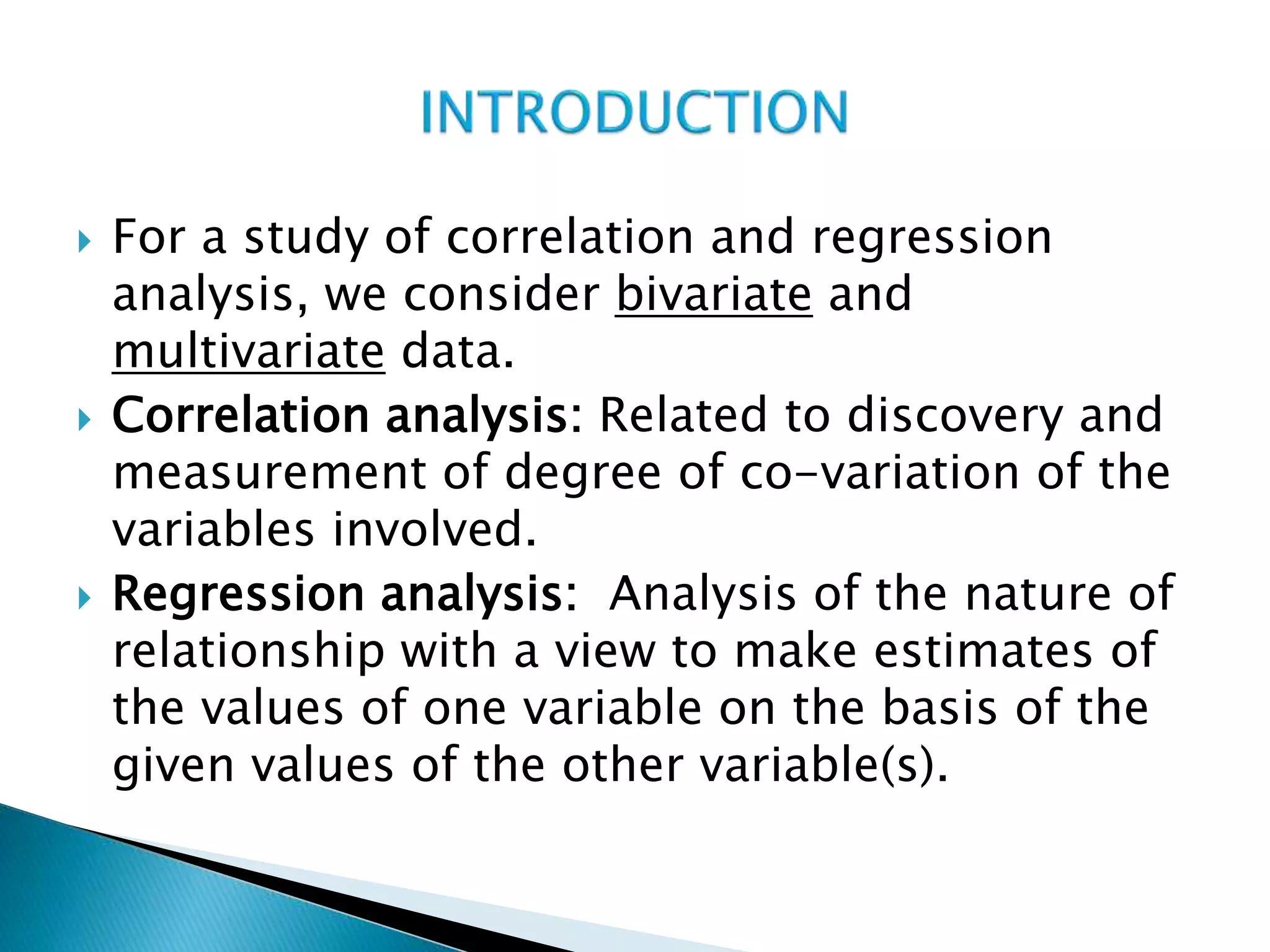
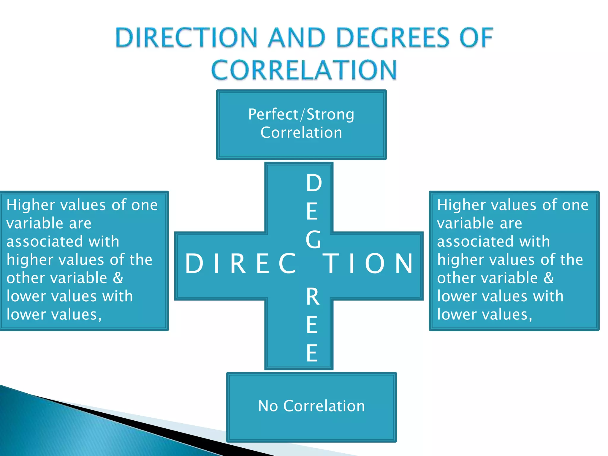
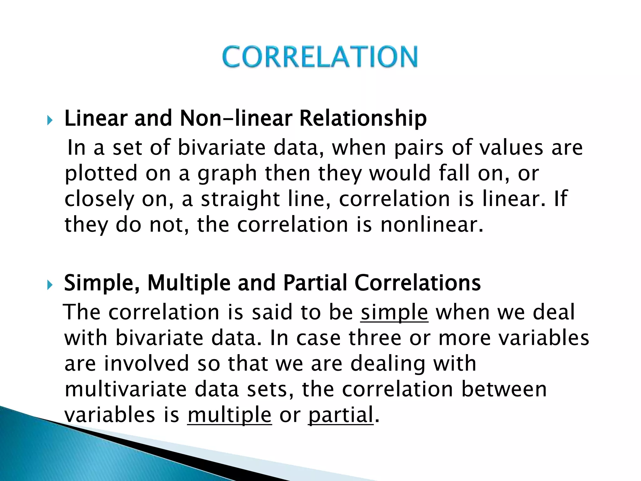
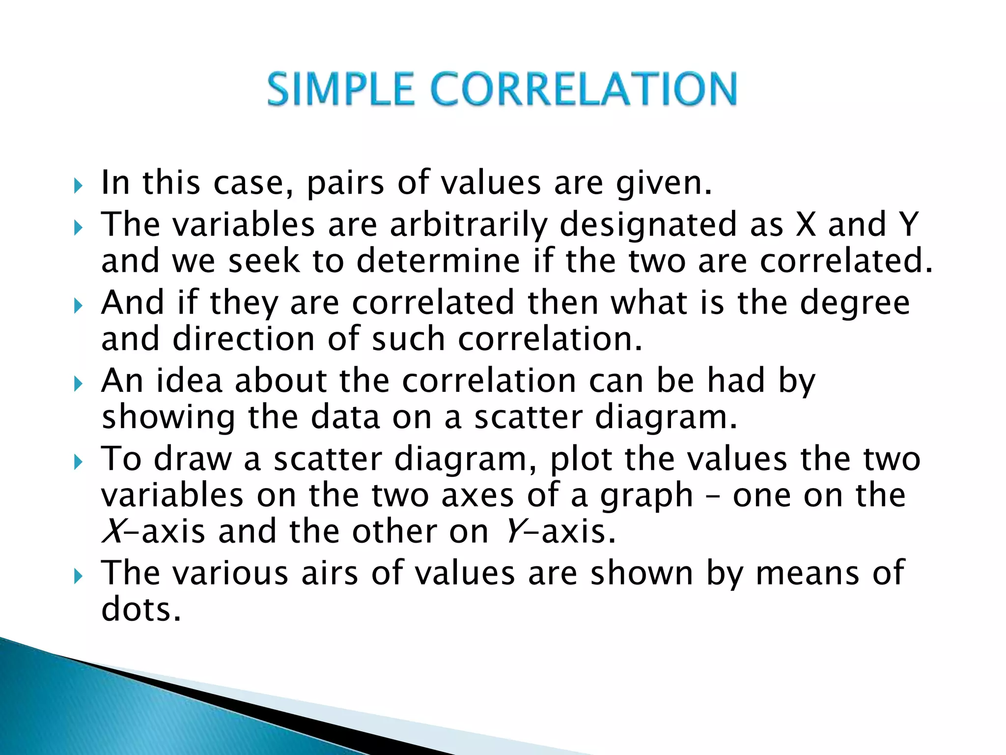
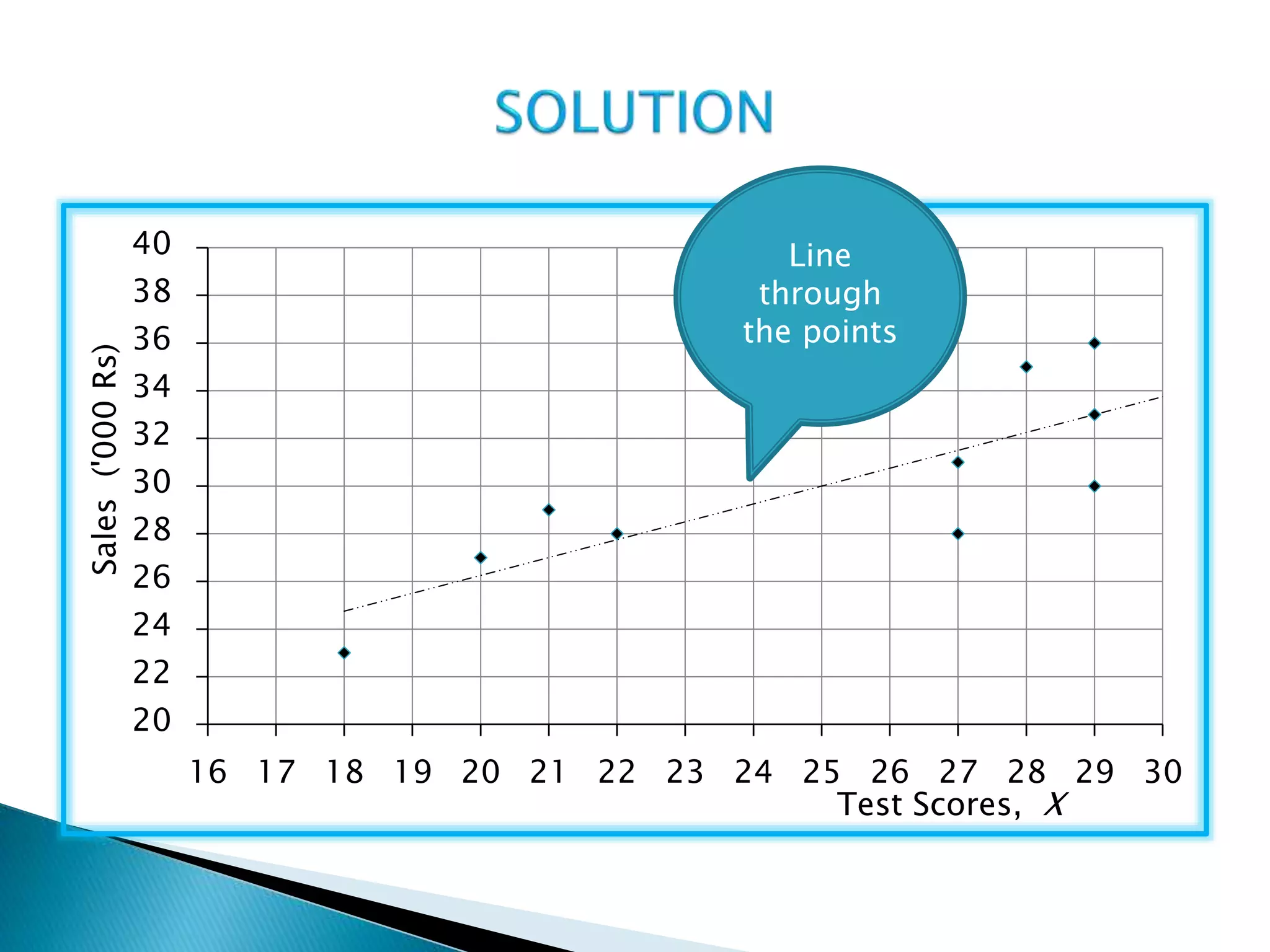
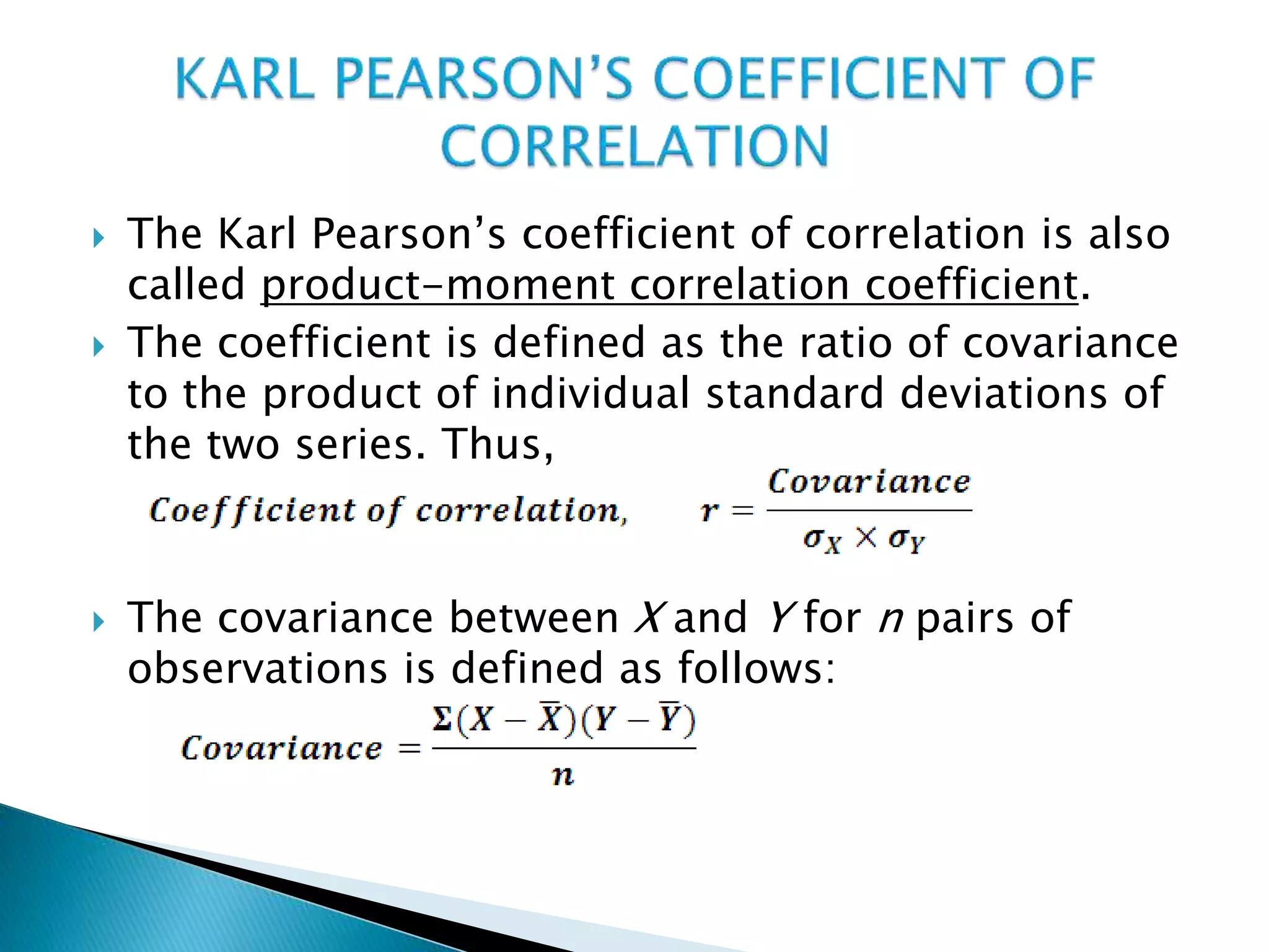
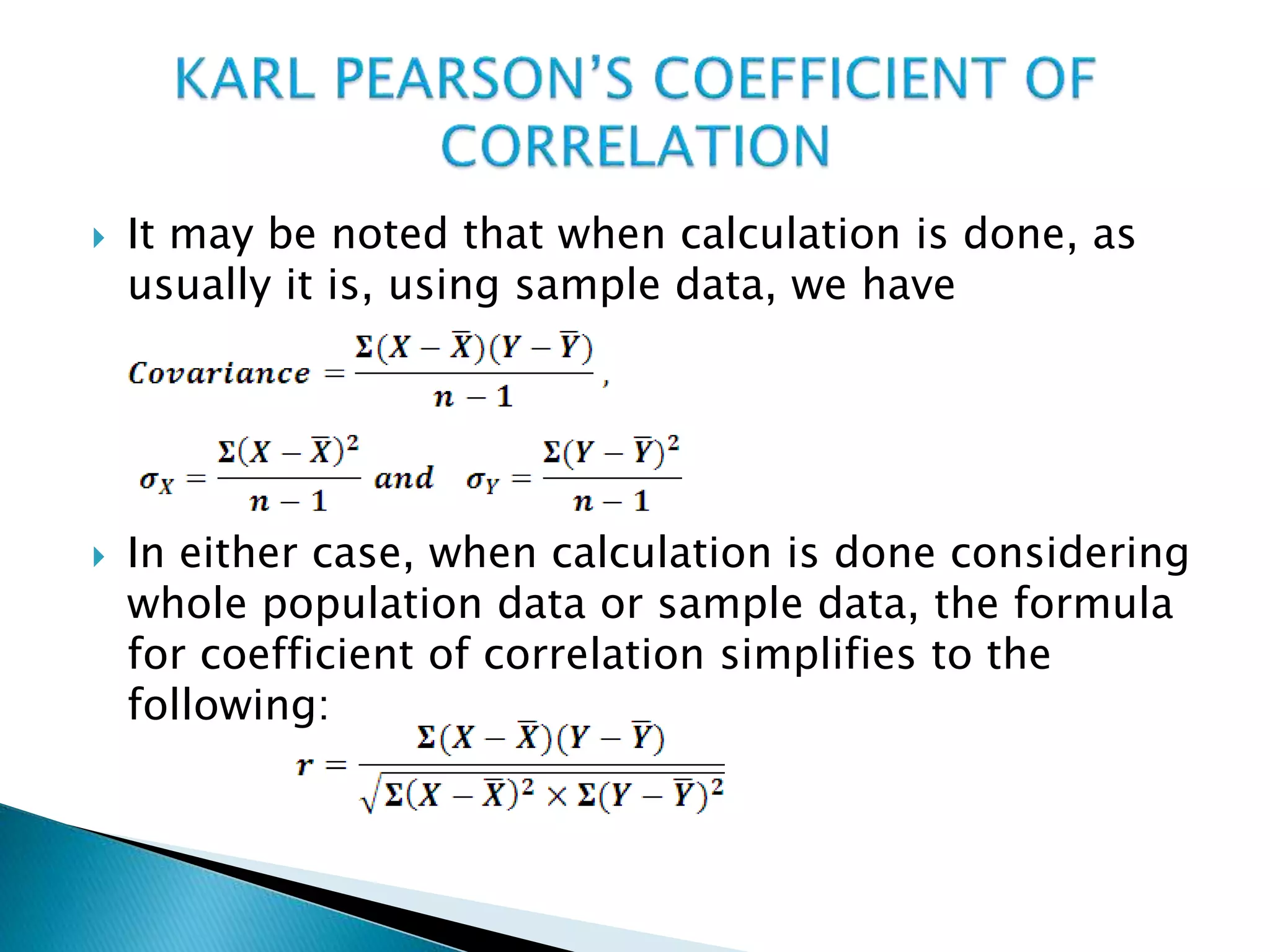
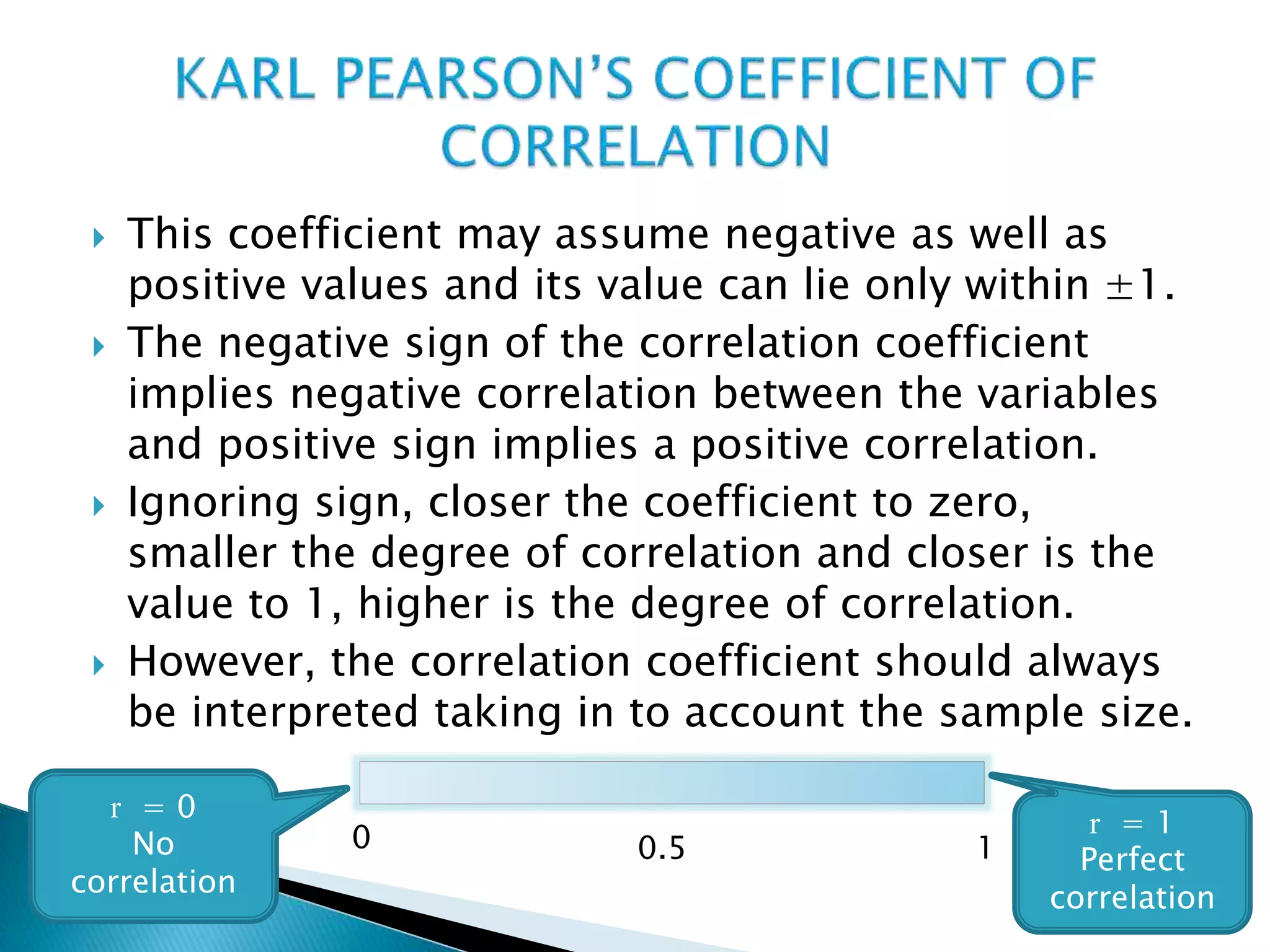
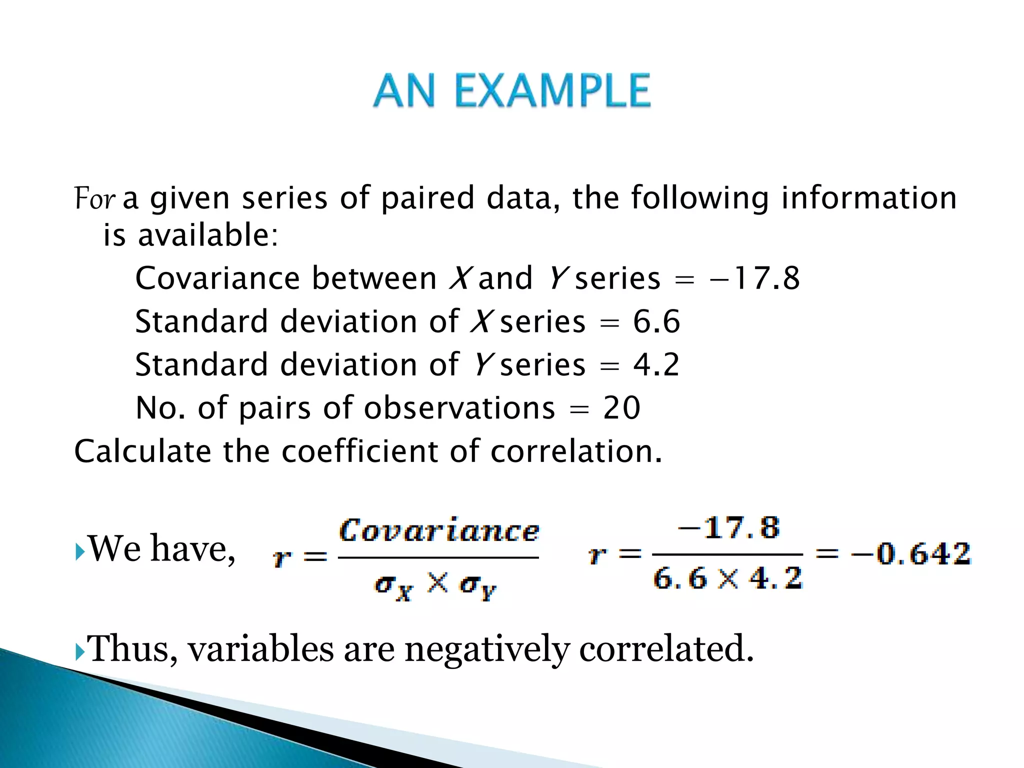
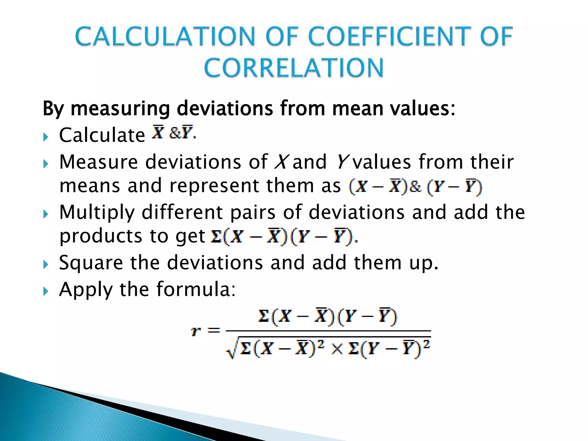
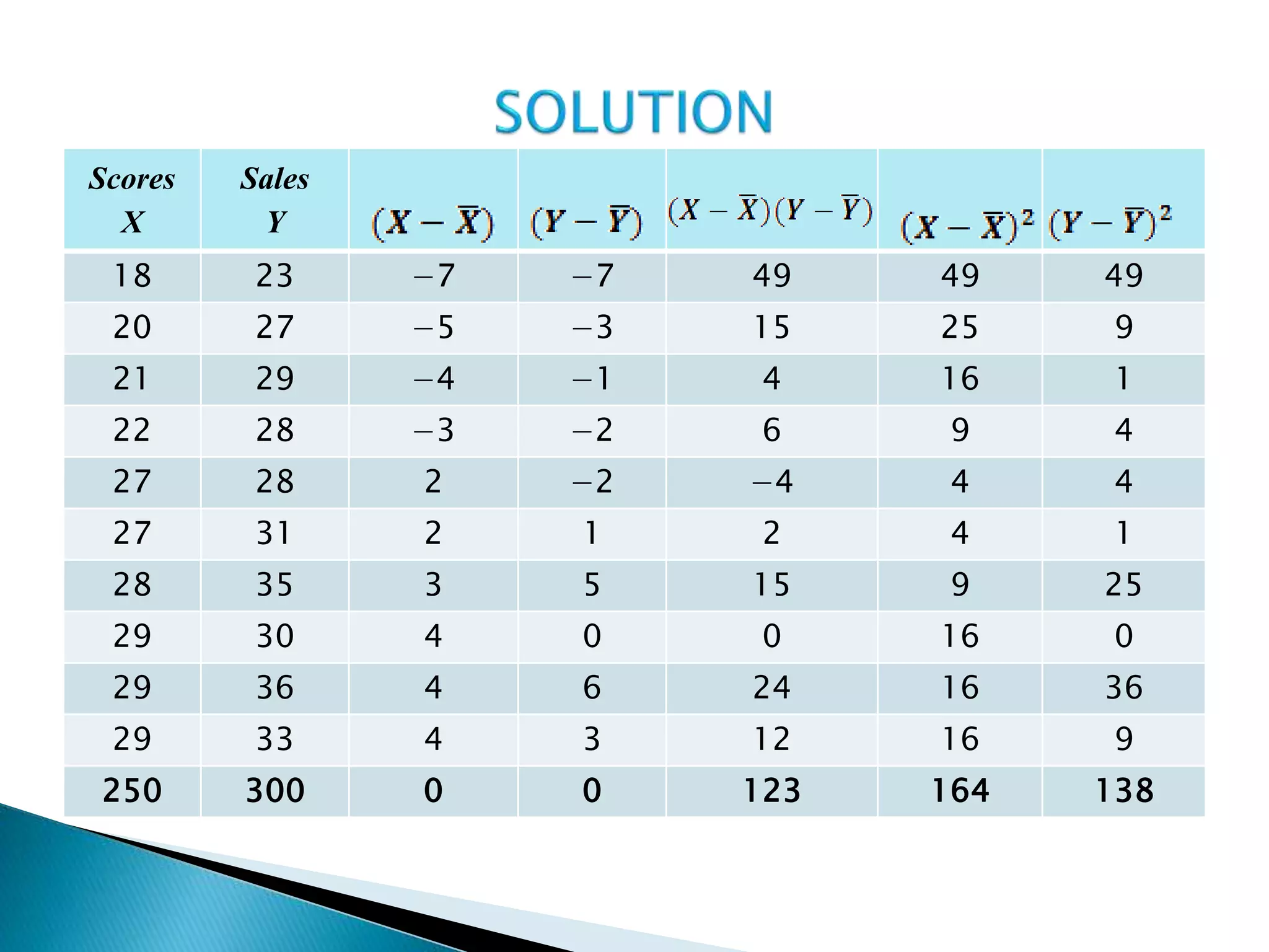
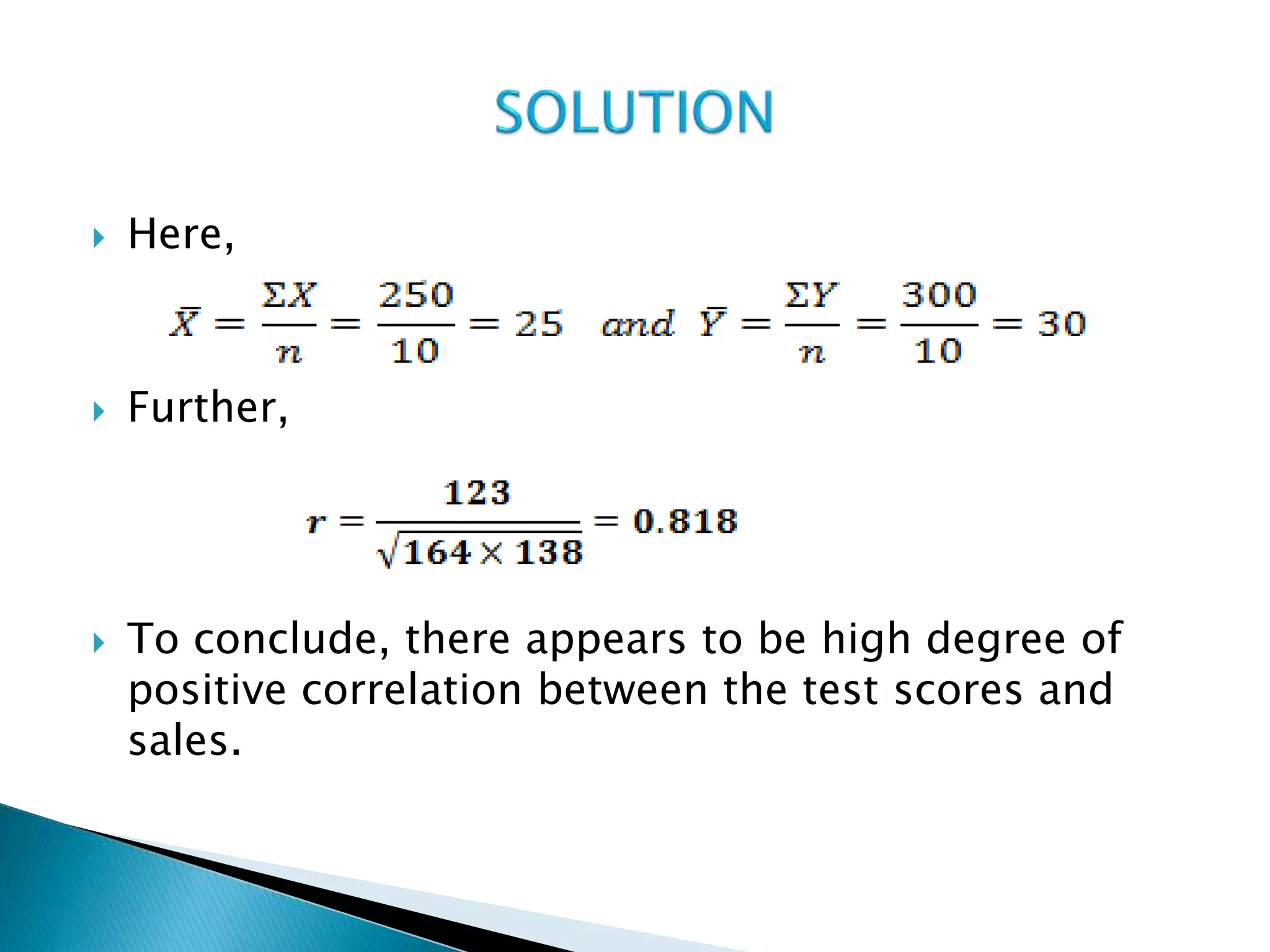
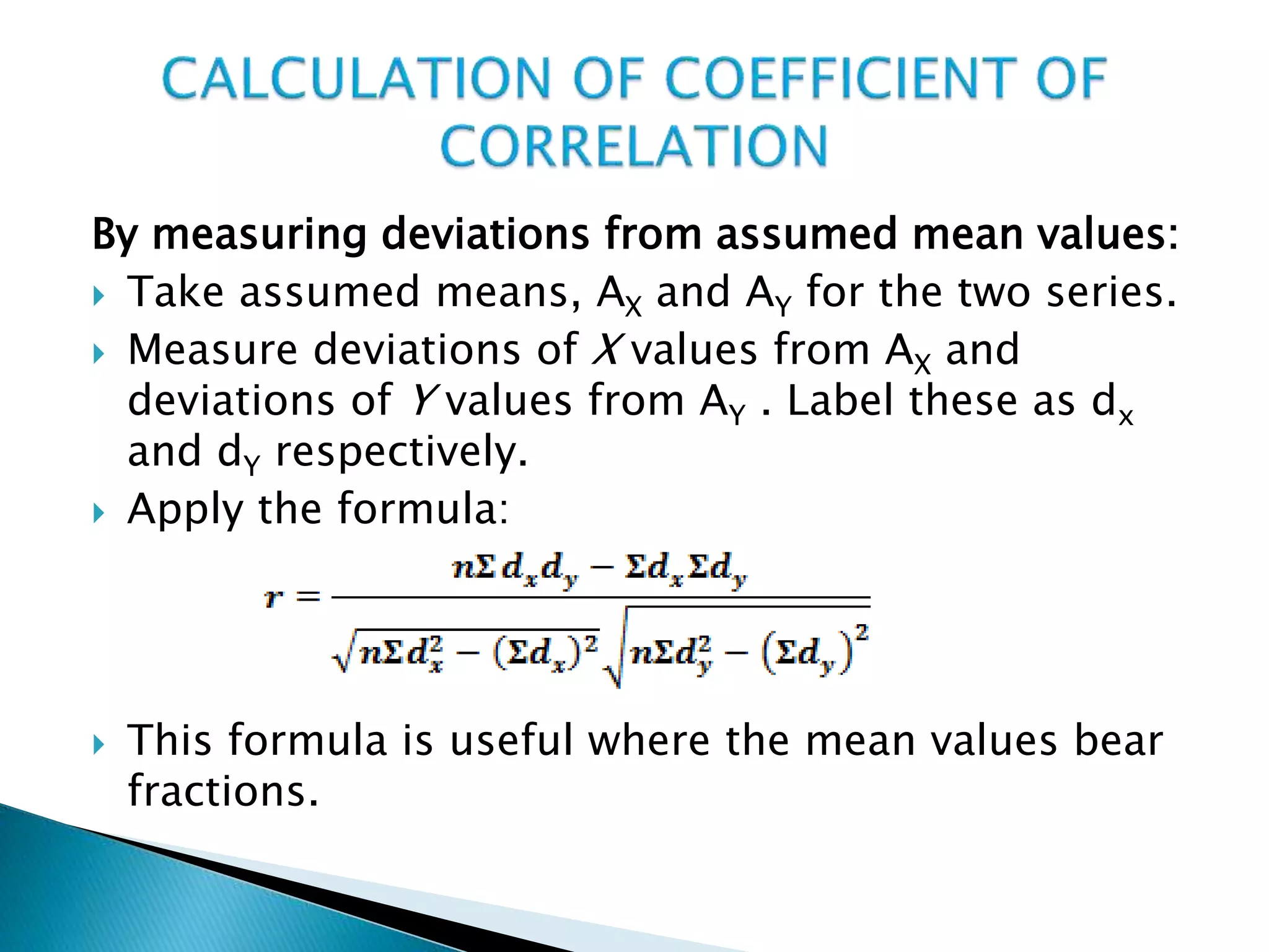
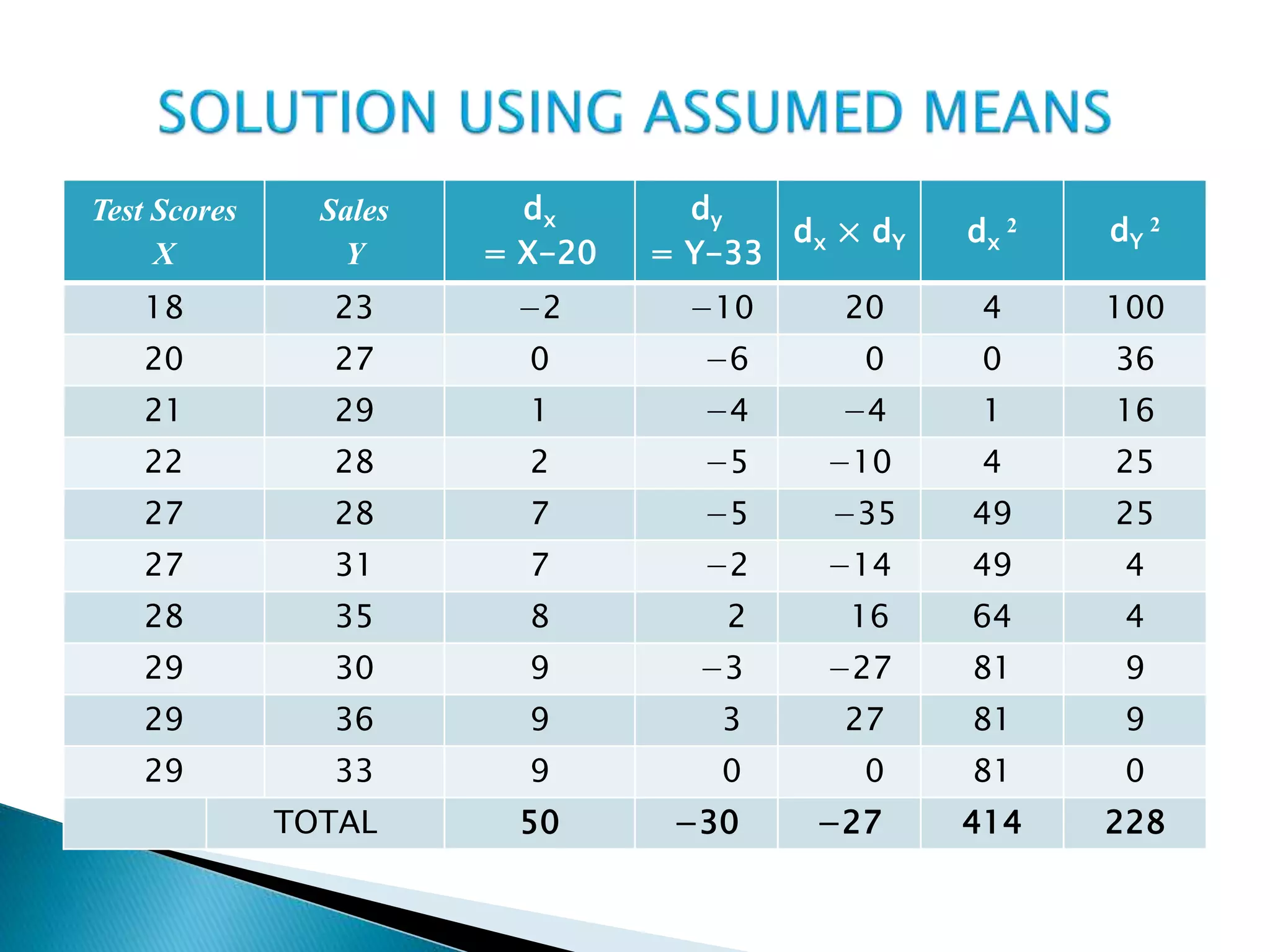
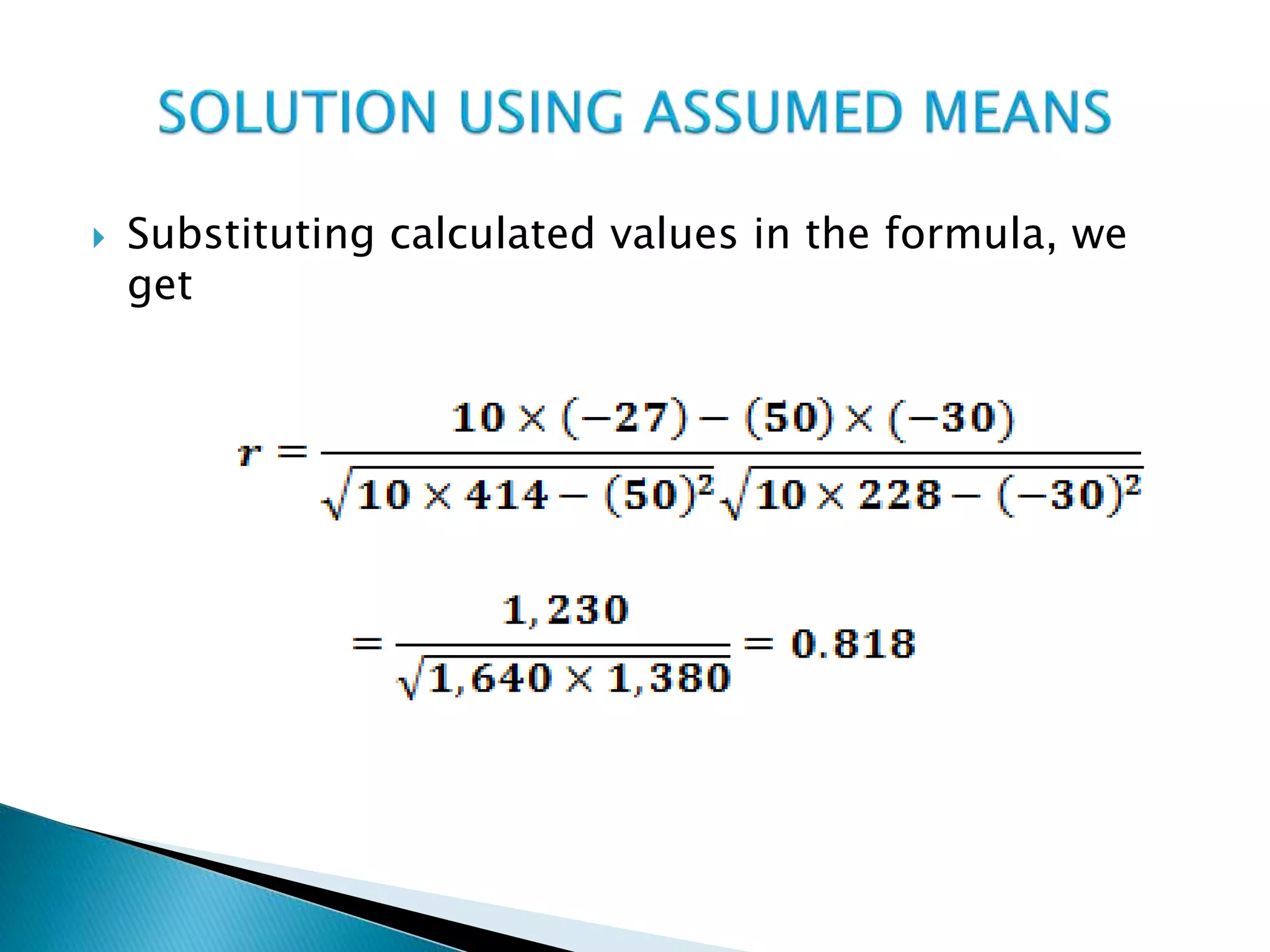
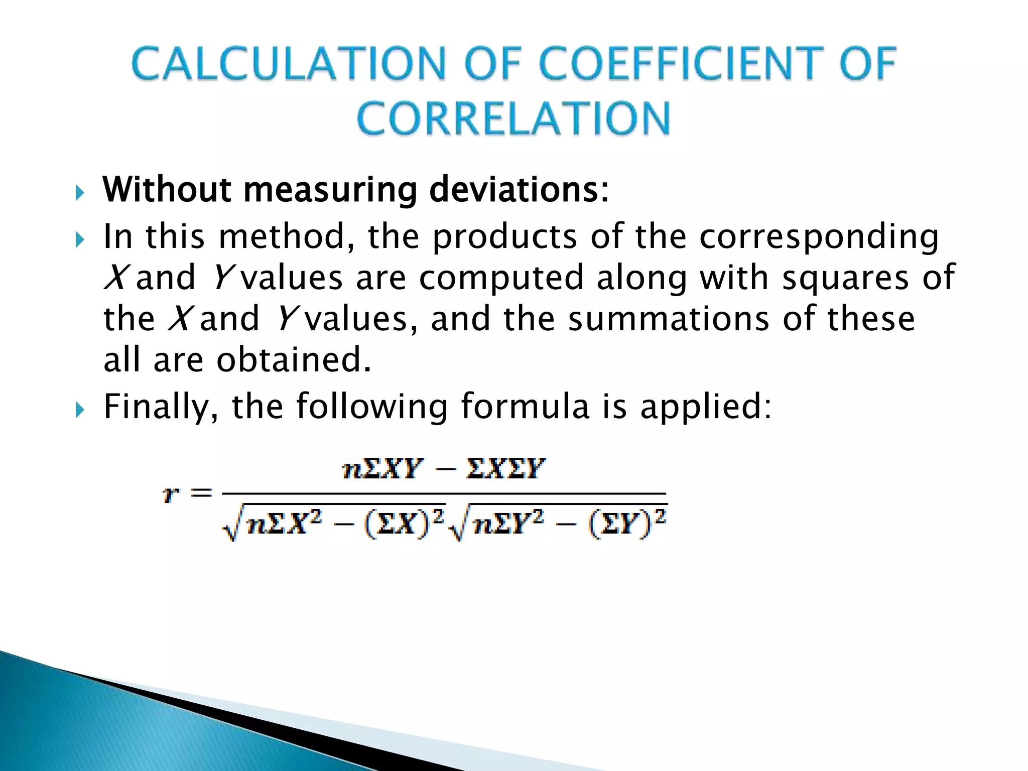
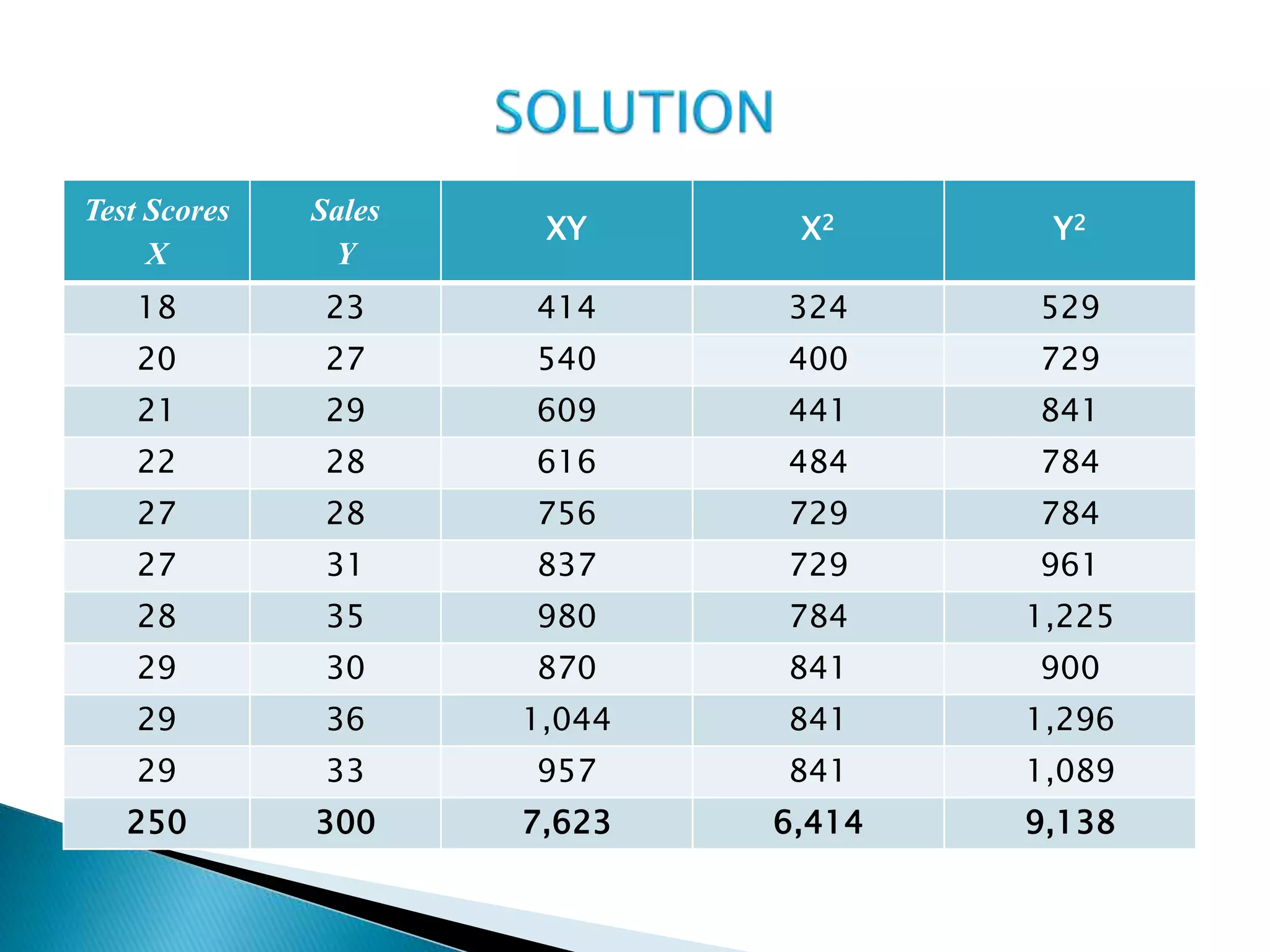
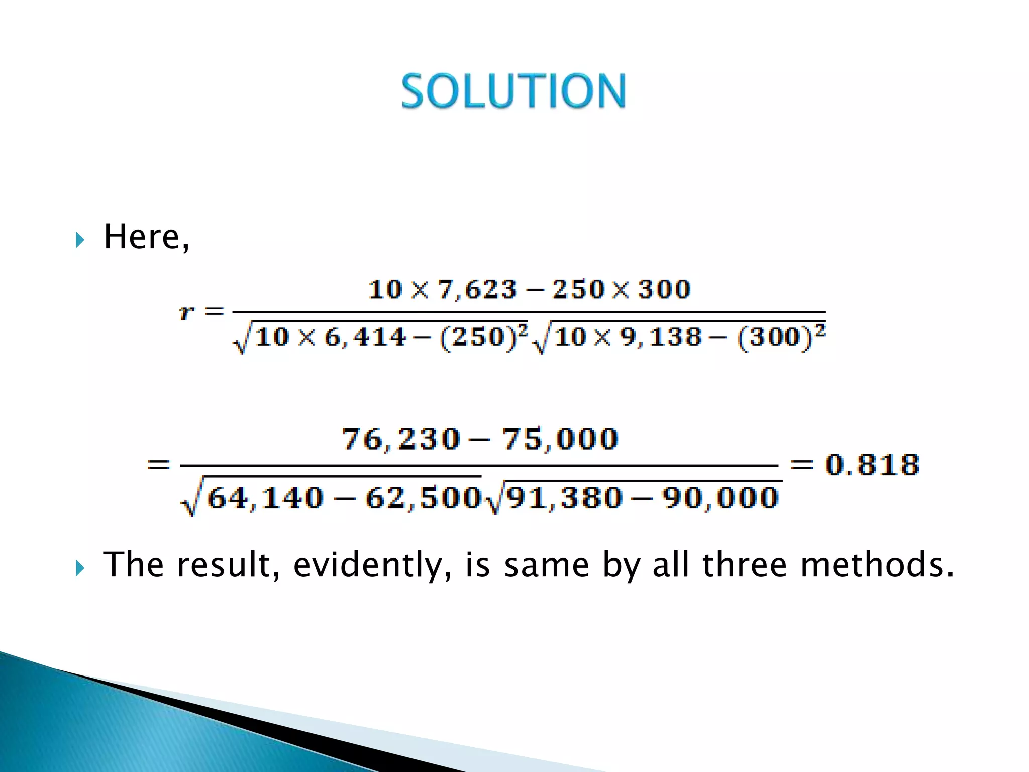
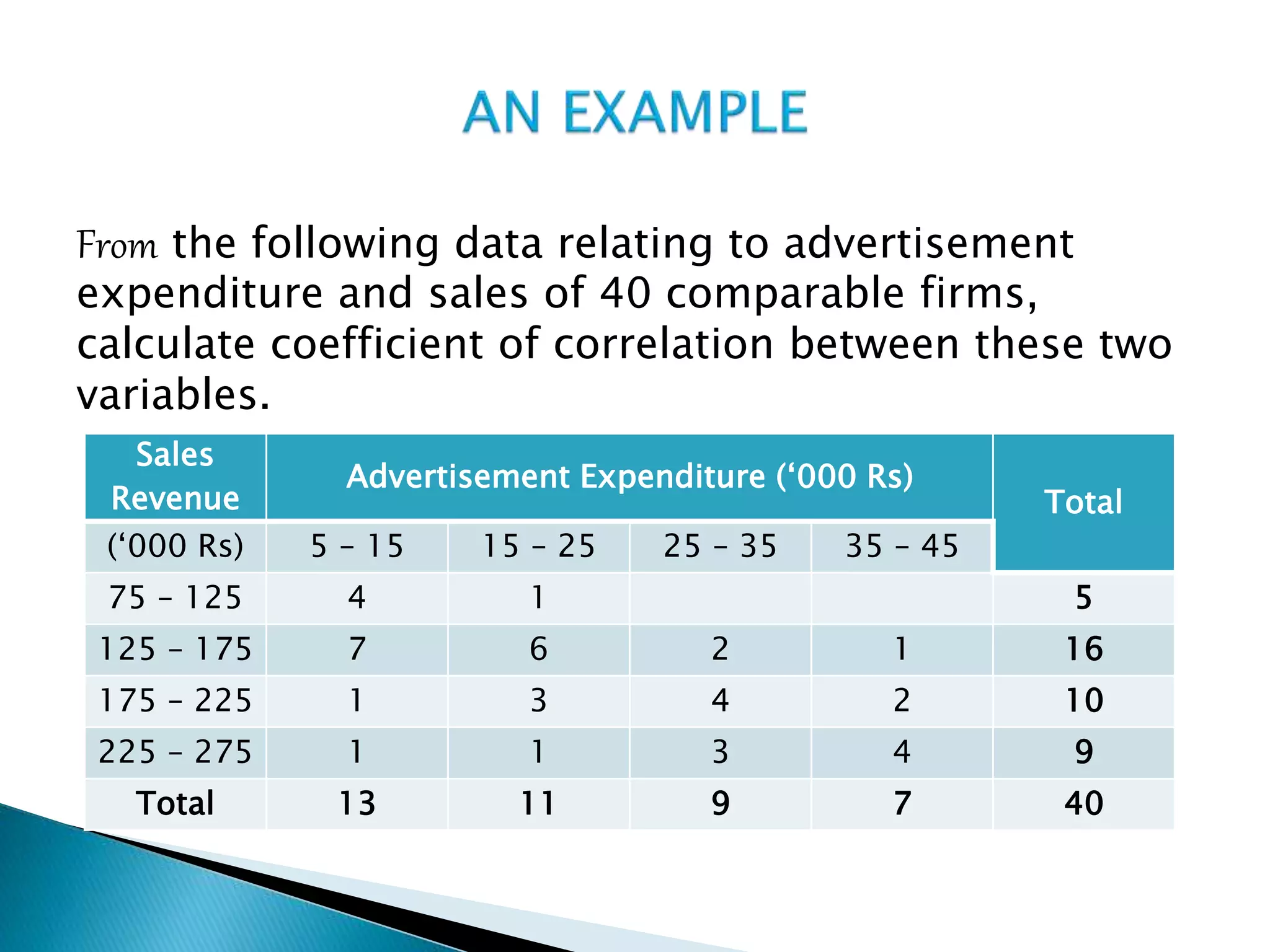
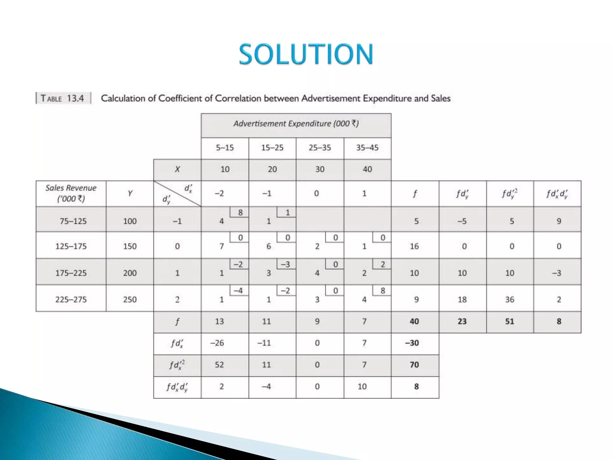
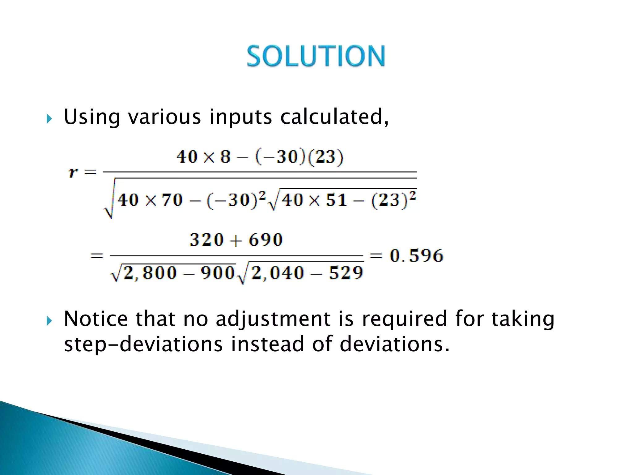
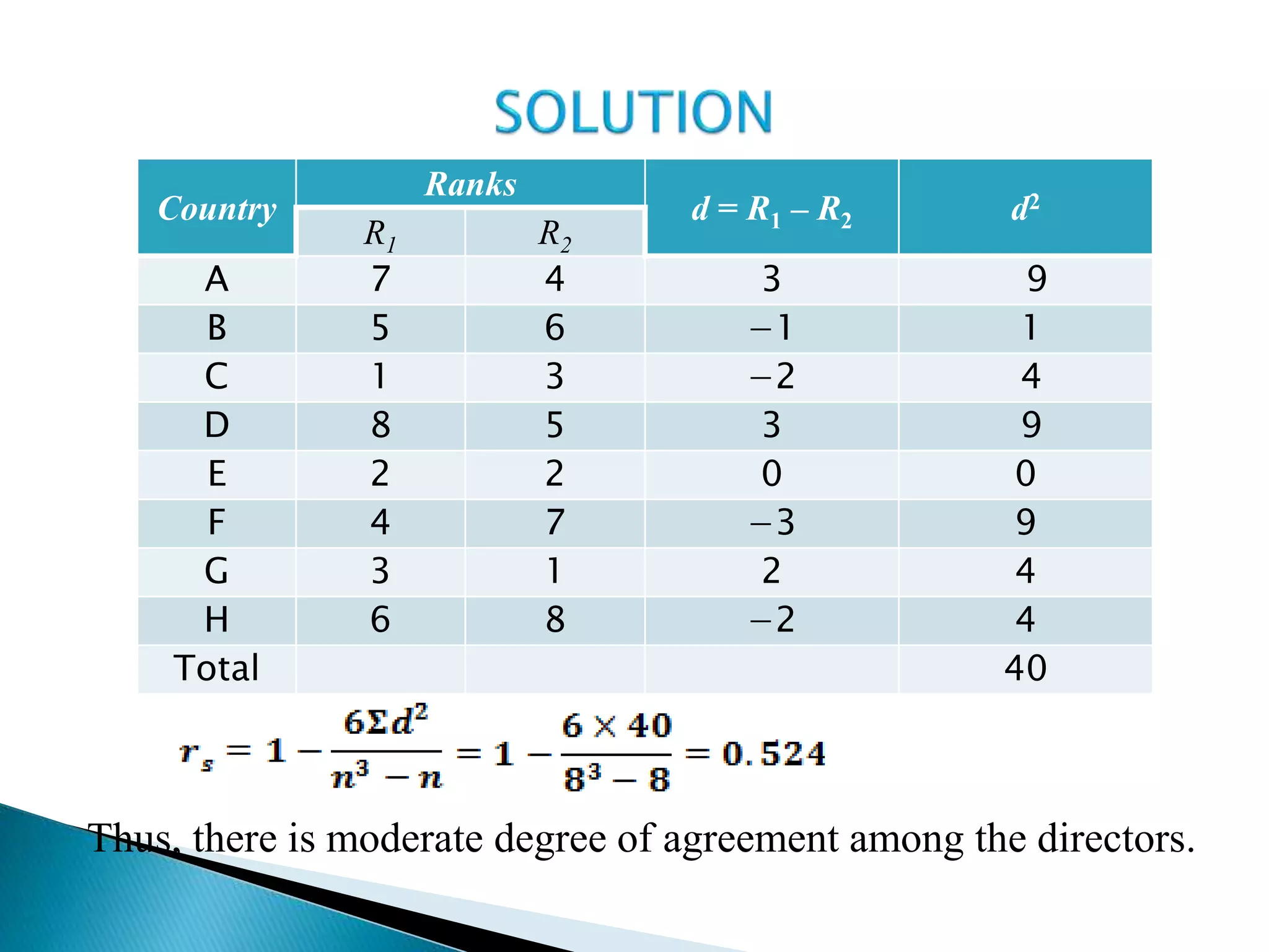
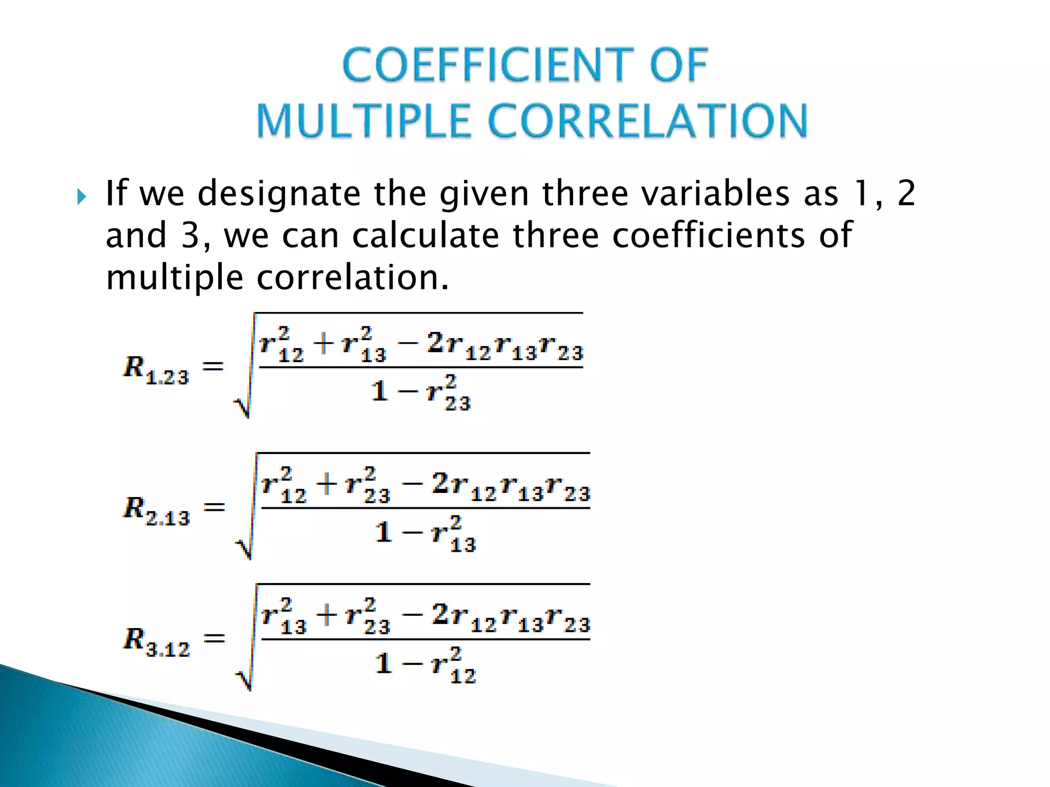
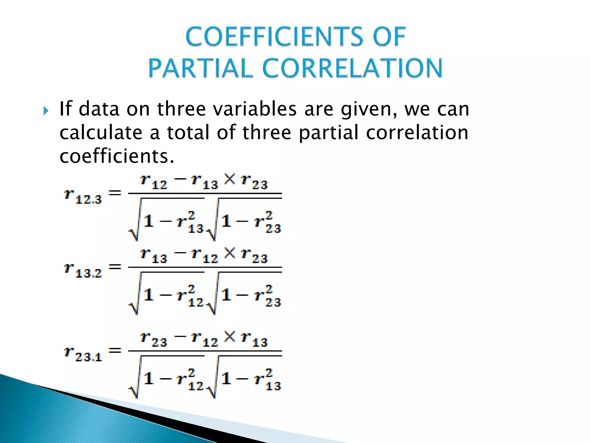
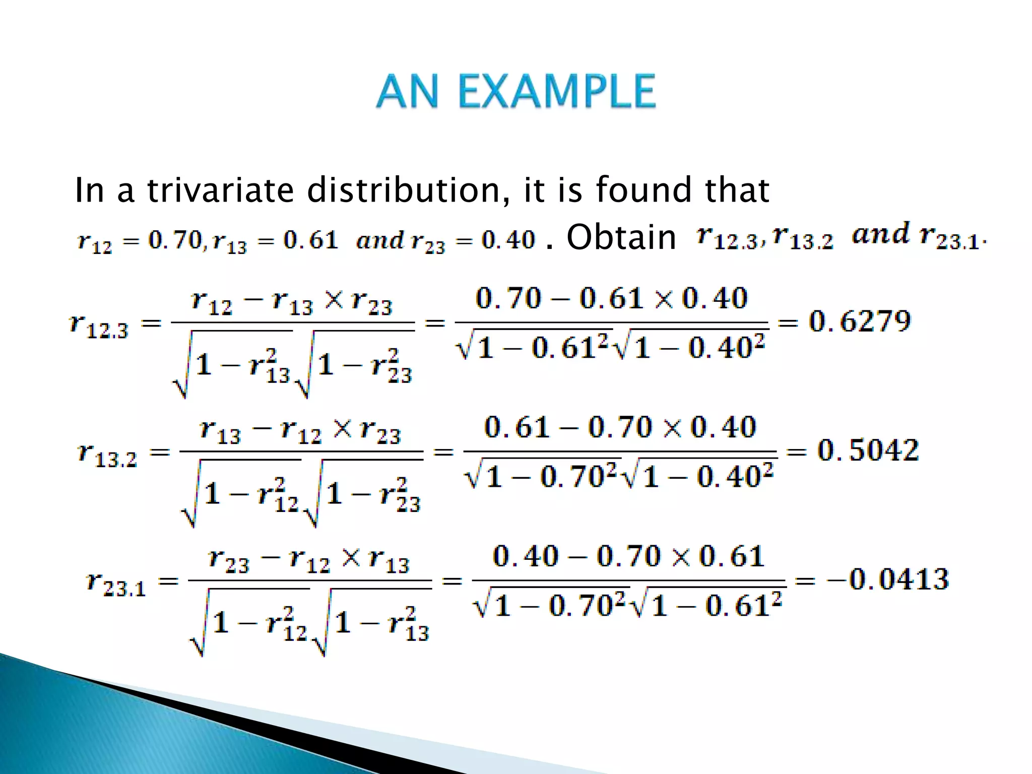
BUSINESS STATISTICS
N. D. VOHRA
Chapter 13
Correlation Analysis
Classification
of Statistical
data
One
variable
Univariate
More than
one variable
Bivariate (Two
Variables)
Multivariate
(more than
two variables)
 For a study of correlation and regression
analysis, we consider bivariate and
multivariate data.
 Correlation analysis: Related to discovery and
measurement of degree of co-variation of the
variables involved.
 Regression analysis: Analysis of the nature of
relationship with a view to make estimates of
the values of one variable on the basis of the
given values of the other variable(s).
 Bivariate Data : When two variables move in sympathy
with each other so that changes in one variable are
associated with changes in the other variable in the
same, or in the opposite direction, they are said to be
correlated.
 When the variables move in same direction, then the
correlation is said to be positive while if they are in
the opposite directions, the correlation is said to be
negative.
 Remember that the direction of movement indicated
is in general. It means that it is not necessary that in
positive correlation a higher value of one variable
shall necessarily be accompanied by a higher value of
the other.
D I R E C T I O N
Higher values of one
variable are
associated with
higher values of the
other variable &
lower values with
lower values,
Higher values of one
variable are
associated with
higher values of the
other variable &
lower values with
lower values,
Perfect/Strong
Correlation
No Correlation
D
E
G
R
E
E
 Linear and Non-linear Relationship
In a set of bivariate data, when pairs of values are
plotted on a graph then they would fall on, or
closely on, a straight line, correlation is linear. If
they do not, the correlation is nonlinear.
 Simple, Multiple and Partial Correlations
The correlation is said to be simple when we deal
with bivariate data. In case three or more variables
are involved so that we are dealing with
multivariate data sets, the correlation between
variables is multiple or partial.
 In this case, pairs of values are given.
 The variables are arbitrarily designated as X and Y
and we seek to determine if the two are correlated.
 And if they are correlated then what is the degree
and direction of such correlation.
 An idea about the correlation can be had by
showing the data on a scatter diagram.
 To draw a scatter diagram, plot the values the two
variables on the two axes of a graph – one on the
X-axis and the other on Y-axis.
 The various airs of values are shown by means of
dots.
 While moving to right on the X-axis, if various dots
are found to be lying higher and higher on the
graph, the correlation between variables is positive.
On the other hand, if they are observed to be lying
lower and lower, then the correlation is negative.
 If various dots may be joined by a straight line,
sloping upward or downward, the correlation is
said to be perfect. The correlation is positive or
negative accordingly as the line is sloping upward
or downward.
 If the dots do not fall exactly on a line but are very
close to being on a line, then there is a high degree
of correlation.
 The more scattered are the dots, the smaller is the
degree of correlation between the variables.
 There is no correlation between the variables when
 the dots are so scattered that there is no clear
direction of their slope, and
 the dots are falling on a line that is parallel to the
X-axis or the Y-axis.
A line parallel to the X-axis implies that the
variable Y is not responsive to changes in X
whereas a line parallel to the Y-axis implies that X
is not sensitive to changes in Y.
Hence there is no correlation in either case.
At National Company the newly recruited salesmen are
given a training which is followed by an aptitude test
before they are put on the job.
The following data collected by the sales manager of the
company shows the scores at the aptitude test and sales
made in the first quarter of their employment by a total of
10 salesmen.
Plot these data on a graph as a scatter diagram and
establish whether correlation exists between the test
scores and sales.
Salesman: 1 2 3 4 5 6 7 8 9 10
Test scores: 18 20 21 22 27 27 28 29 29 29
Sales (000 Rs): 23 27 29 28 28 31 35 30 36 33
20
22
24
26
28
30
32
34
36
38
40
16 17 18 19 20 21 22 23 24 25 26 27 28 29 30
Test Scores, X
Sales('000Rs)
Line
through
the points
 The Karl Pearson’s coefficient of correlation is also
called product-moment correlation coefficient.
 The coefficient is defined as the ratio of covariance
to the product of individual standard deviations of
the two series. Thus,
 The covariance between X and Y for n pairs of
observations is defined as follows:
 It may be noted that when calculation is done, as
usually it is, using sample data, we have
 In either case, when calculation is done considering
whole population data or sample data, the formula
for coefficient of correlation simplifies to the
following:
 This coefficient may assume negative as well as
positive values and its value can lie only within ±1.
 The negative sign of the correlation coefficient
implies negative correlation between the variables
and positive sign implies a positive correlation.
 Ignoring sign, closer the coefficient to zero,
smaller the degree of correlation and closer is the
value to 1, higher is the degree of correlation.
 However, the correlation coefficient should always
be interpreted taking in to account the sample size.
0 1
r = 0
No
correlation
r = 1
Perfect
correlation
0.5
For a given series of paired data, the following information
is available:
Covariance between X and Y series = −17.8
Standard deviation of X series = 6.6
Standard deviation of Y series = 4.2
No. of pairs of observations = 20
Calculate the coefficient of correlation.
We have,
Thus, variables are negatively correlated.
By measuring deviations from mean values:
 Calculate
 Measure deviations of X and Y values from their
means and represent them as
 Multiply different pairs of deviations and add the
products to get
 Square the deviations and add them up.
 Apply the formula:
At National Company the newly recruited salesmen are
given a training which is followed by an aptitude test
before they are put on the job.
The following data collected by the sales manager of
the company shows the scores at the aptitude test
and sales made in the first quarter of their
employment by a total of 10 salesmen.
Calculate coefficient of correlation
Salesman: 1 2 3 4 5 6 7 8 9 10
Test scores: 18 20 21 22 27 27 28 29 29 29
Sales (000 Rs): 23 27 29 28 28 31 35 30 36 33
Scores
X
Sales
Y
18 23 −7 −7 49 49 49
20 27 −5 −3 15 25 9
21 29 −4 −1 4 16 1
22 28 −3 −2 6 9 4
27 28 2 −2 −4 4 4
27 31 2 1 2 4 1
28 35 3 5 15 9 25
29 30 4 0 0 16 0
29 36 4 6 24 16 36
29 33 4 3 12 16 9
250 300 0 0 123 164 138
 Here,
 Further,
 To conclude, there appears to be high degree of
positive correlation between the test scores and
sales.
By measuring deviations from assumed mean values:
 Take assumed means, AX and AY for the two series.
 Measure deviations of X values from AX and
deviations of Y values from AY . Label these as dx
and dY respectively.
 Apply the formula:
 This formula is useful where the mean values bear
fractions.
Test Scores
X
Sales
Y
dx
= X-20
dy
= Y-33
dx × dY dx
2 dY
2
18 23 −2 −10 20 4 100
20 27 0 −6 0 0 36
21 29 1 −4 −4 1 16
22 28 2 −5 −10 4 25
27 28 7 −5 −35 49 25
27 31 7 −2 −14 49 4
28 35 8 2 16 64 4
29 30 9 −3 −27 81 9
29 36 9 3 27 81 9
29 33 9 0 0 81 0
TOTAL 50 −30 −27 414 228
 Substituting calculated values in the formula, we
get
 Without measuring deviations:
 In this method, the products of the corresponding
X and Y values are computed along with squares of
the X and Y values, and the summations of these
all are obtained.
 Finally, the following formula is applied:
Test Scores
X
Sales
Y
XY X2 Y2
18 23 414 324 529
20 27 540 400 729
21 29 609 441 841
22 28 616 484 784
27 28 756 729 784
27 31 837 729 961
28 35 980 784 1,225
29 30 870 841 900
29 36 1,044 841 1,296
29 33 957 841 1,089
250 300 7,623 6,414 9,138
 Here,
 The result, evidently, is same by all three methods.
 Name the two variables as X and Y.
 Now, find mid-points of the different classes for both
the variables.
 Take deviations, or step-deviations, from assumed
mean values in respect of each of the variables and
label these as dx and dY respectively.
 Have three columns headed fdY fdY
2, fdY dx and three
rows headed fdx, fdx
2 and fdY dx.
 Multiply marginal frequencies ( total of cell frequencies)
with dY dY
2, and enter these products in appropriate
columns. Repeat the process for each of the columns
and enter the products in appropriate rows.
 Obtain the summations of all.
 Consider each cell frequency individually and
obtain from northward the value of dx and from
westward the value of dY.
 Multiply all the three to get and place the products
in respective cells in their top right hand corners.
 These values are then added up across the columns
for each row and placed in the column headed fdY
dx . Similarly, these are totaled up down each
column and put in the row labeled fdY dx .
 Now,
From the following data relating to advertisement
expenditure and sales of 40 comparable firms,
calculate coefficient of correlation between these two
variables.
Sales
Revenue
Advertisement Expenditure (‘000 Rs)
Total
(‘000 Rs) 5 – 15 15 – 25 25 – 35 35 – 45
75 – 125 4 1 5
125 – 175 7 6 2 1 16
175 – 225 1 3 4 2 10
225 – 275 1 1 3 4 9
Total 13 11 9 7 40
 Using various inputs calculated,
 Notice that no adjustment is required for taking
step-deviations instead of deviations.
 Linear Relationship: The product-moment
coefficient of correlation assumes essentially that
the relationship between the variables is linear in
nature.
 Normality: A further assumption is that a large
number of independent factors operate on each of
the variables being correlated in such a way that
each of them is normally distributed.
 The Karl Pearson’s coefficient of correlation is a
pure number and is divorced of the units in which
the original data are expressed.
 As indicated earlier, the value of the coefficient of
correlation varies between ±1.
 The coefficient of correlation is independent of the
change of origin and scale of the data. Thus, if a
constant is added to/subtracted from one or both
variable values or if all values are multiplied or
divided by a constant, it will have no effect on the
value of the coefficient.
 Null hypothesis, H0: ρ = 0 (Correlation in the
population is zero)
 Alternate hypothesis, H1: ρ ≠ 0 (Correlation in the
population is other than zero)
 Level of significance, α = 0.05 (say)
 Test statistic:
The data of 10 sales manager of the National
Company showed the correlation between test scores
and the sales made by salesmen to be equal to 0.818.
This suggested a strong correlation between the two
variables.
Test the significance of correlation coefficient.
 Null hypothesis, H0: ρ =
 Alternate hypothesis, H1: ρ ≠ 0
 Level of significance, α = 0.05 (say)
 Test statistic: t
 Decision Rule: If , reject the null hypothesis
 Computations:
 Conclusion: The null hypothesis is rejected at 0.05
level of significance meaning thereby that the
correlation in the population is not zero. From the
practical standpoint, it indicates for the sales
manager that there is correlation in the population
of salespersons with respect to their test scores and
sales made by them.
 Sometimes probable error is used in interpreting a
correlation coefficient, r. The probable error, PE, is
defined as follows:
 The correlation coefficient is considered to be
significant when it exceeds 6 times the probable error.
 It may be noted that the value of probable error is
related inversely to the value of n so that smaller the
value of n greater is the probable error for a given value
of r.
 It measures how much variation in one variable is
explained by variation in the other variable.
 It is numerically equal to the square of the
coefficient of correlation, r2.
 An r2 equal to 0.64 implies that 64 percent of the
variation in one variable is due to variation in the
other variable.
 In the context of a situation where the variables are
perfectly correlated so that r = 1 (or −1). In such a
case, r2 = 1 implies that all changes in one variable
are explained by changes in the other variable.
 First, too much importance may not be given to
coefficients of correlation obtained from small data
sets as they may lead to erroneous conclusions.
 In any case, it is always advisable to interpret the
value of a given correlation coefficient using the
probable error.
 Secondly, it should be clearly understood that while
a cause-and-effect relationship between two
variables would result in a correlation between
them the reverse is not true.
 Further, sometimes a high correlation may be
found between the variables due to chance alone.
 Rank correlation is calculated essentially where the
variables under consideration cannot quantified
being measured on ordinal scale.
 However, it can be calculated even where the
variables are objectively quantifiable.
 This is done by ranking the given data on the basis
of the values involved.
 The rank correlation coefficient also varies between
±1.
 The presence of extreme observations in the data
does not distort the value of rank correlation
coefficient.
 Let there be n pairs of values of two ranked
variables, or two rankings of a variable.
 The ranks may already be given or else they may be
obtained by ranking the given values as 1, 2,, … , n
in ascending or descending order.
 Now, find the difference, d, between different pairs
of ranks and obtain their squares, d2.
 Finally, obtain the summation of the squared
differences, and apply the formula:
Eight countries were ranked by two directors of a
company seeking to expand its activities in the
foreign markets in terms of their sales potential.
Determine to what extent is the assessment of the
two directors agreed.
Country: A B C D E F G H
Ranking
by
Director 1: 7 5 1 8 2 4 3 6
Director 2: 4 6 3 5 2 7 1 8
Country
Ranks
d = R1 – R2 d2
R1 R2
A 7 4 3 9
B 5 6 −1 1
C 1 3 −2 4
D 8 5 3 9
E 2 2 0 0
F 4 7 −3 9
G 3 1 2 4
H 6 8 −2 4
Total 40
Thus, there is moderate degree of agreement among the directors.
 While ranking, it may sometimes not be possible to
distinguish clearly between adjacent units.
 The ranks are said to be tied in such a case.
 Similarly, in quantitatively expressed data, tied
ranks are experienced when equal values appear in
a given series.
 The problem is resolved by assigning the average
of the ranks involved to each of them.
 If there are m items with common ranks, then a
value equal to (m3-m)/12 is added to sum of
square of difference as a correction factor for
calculating coefficient of correlation.
 If there is more than one such group of items with
common ranks, the correction factor is added as
many times as the number of groups.
 The coefficient of rank correlation is given by:
 When the data involve two variables, the correlation
between the variables is called simple correlation
 When they involve more than two variables, then we
study multiple and partial correlations.
 In such data, there are two or more independent
variables which affect a dependent variable.
 Multiple correlation is used to study the joint or
cumulative effect of all the given independent
variables on the dependent variable.
 The partial correlation involves a study of correlation
between one independent variable and the dependent
variable holding the other independent variable(s)
constant statistically.
 If we designate the given three variables as 1, 2
and 3, we can calculate three coefficients of
multiple correlation.
 If data on three variables are given, we can
calculate a total of three partial correlation
coefficients.
In a trivariate distribution, it is found that
. Obtain
END OF CHAPTER 13

data analysis

  • 1.
    BUSINESS STATISTICS N. D.VOHRA Chapter 13 Correlation Analysis
  • 2.
    Classification of Statistical data One variable Univariate More than onevariable Bivariate (Two Variables) Multivariate (more than two variables)
  • 3.
     For astudy of correlation and regression analysis, we consider bivariate and multivariate data.  Correlation analysis: Related to discovery and measurement of degree of co-variation of the variables involved.  Regression analysis: Analysis of the nature of relationship with a view to make estimates of the values of one variable on the basis of the given values of the other variable(s).
  • 4.
     Bivariate Data: When two variables move in sympathy with each other so that changes in one variable are associated with changes in the other variable in the same, or in the opposite direction, they are said to be correlated.  When the variables move in same direction, then the correlation is said to be positive while if they are in the opposite directions, the correlation is said to be negative.  Remember that the direction of movement indicated is in general. It means that it is not necessary that in positive correlation a higher value of one variable shall necessarily be accompanied by a higher value of the other.
  • 5.
    D I RE C T I O N Higher values of one variable are associated with higher values of the other variable & lower values with lower values, Higher values of one variable are associated with higher values of the other variable & lower values with lower values, Perfect/Strong Correlation No Correlation D E G R E E
  • 6.
     Linear andNon-linear Relationship In a set of bivariate data, when pairs of values are plotted on a graph then they would fall on, or closely on, a straight line, correlation is linear. If they do not, the correlation is nonlinear.  Simple, Multiple and Partial Correlations The correlation is said to be simple when we deal with bivariate data. In case three or more variables are involved so that we are dealing with multivariate data sets, the correlation between variables is multiple or partial.
  • 7.
     In thiscase, pairs of values are given.  The variables are arbitrarily designated as X and Y and we seek to determine if the two are correlated.  And if they are correlated then what is the degree and direction of such correlation.  An idea about the correlation can be had by showing the data on a scatter diagram.  To draw a scatter diagram, plot the values the two variables on the two axes of a graph – one on the X-axis and the other on Y-axis.  The various airs of values are shown by means of dots.
  • 8.
     While movingto right on the X-axis, if various dots are found to be lying higher and higher on the graph, the correlation between variables is positive. On the other hand, if they are observed to be lying lower and lower, then the correlation is negative.  If various dots may be joined by a straight line, sloping upward or downward, the correlation is said to be perfect. The correlation is positive or negative accordingly as the line is sloping upward or downward.  If the dots do not fall exactly on a line but are very close to being on a line, then there is a high degree of correlation.
  • 9.
     The morescattered are the dots, the smaller is the degree of correlation between the variables.  There is no correlation between the variables when  the dots are so scattered that there is no clear direction of their slope, and  the dots are falling on a line that is parallel to the X-axis or the Y-axis. A line parallel to the X-axis implies that the variable Y is not responsive to changes in X whereas a line parallel to the Y-axis implies that X is not sensitive to changes in Y. Hence there is no correlation in either case.
  • 11.
    At National Companythe newly recruited salesmen are given a training which is followed by an aptitude test before they are put on the job. The following data collected by the sales manager of the company shows the scores at the aptitude test and sales made in the first quarter of their employment by a total of 10 salesmen. Plot these data on a graph as a scatter diagram and establish whether correlation exists between the test scores and sales. Salesman: 1 2 3 4 5 6 7 8 9 10 Test scores: 18 20 21 22 27 27 28 29 29 29 Sales (000 Rs): 23 27 29 28 28 31 35 30 36 33
  • 12.
    20 22 24 26 28 30 32 34 36 38 40 16 17 1819 20 21 22 23 24 25 26 27 28 29 30 Test Scores, X Sales('000Rs) Line through the points
  • 13.
     The KarlPearson’s coefficient of correlation is also called product-moment correlation coefficient.  The coefficient is defined as the ratio of covariance to the product of individual standard deviations of the two series. Thus,  The covariance between X and Y for n pairs of observations is defined as follows:
  • 14.
     It maybe noted that when calculation is done, as usually it is, using sample data, we have  In either case, when calculation is done considering whole population data or sample data, the formula for coefficient of correlation simplifies to the following:
  • 15.
     This coefficientmay assume negative as well as positive values and its value can lie only within ±1.  The negative sign of the correlation coefficient implies negative correlation between the variables and positive sign implies a positive correlation.  Ignoring sign, closer the coefficient to zero, smaller the degree of correlation and closer is the value to 1, higher is the degree of correlation.  However, the correlation coefficient should always be interpreted taking in to account the sample size. 0 1 r = 0 No correlation r = 1 Perfect correlation 0.5
  • 16.
    For a givenseries of paired data, the following information is available: Covariance between X and Y series = −17.8 Standard deviation of X series = 6.6 Standard deviation of Y series = 4.2 No. of pairs of observations = 20 Calculate the coefficient of correlation. We have, Thus, variables are negatively correlated.
  • 17.
    By measuring deviationsfrom mean values:  Calculate  Measure deviations of X and Y values from their means and represent them as  Multiply different pairs of deviations and add the products to get  Square the deviations and add them up.  Apply the formula:
  • 18.
    At National Companythe newly recruited salesmen are given a training which is followed by an aptitude test before they are put on the job. The following data collected by the sales manager of the company shows the scores at the aptitude test and sales made in the first quarter of their employment by a total of 10 salesmen. Calculate coefficient of correlation Salesman: 1 2 3 4 5 6 7 8 9 10 Test scores: 18 20 21 22 27 27 28 29 29 29 Sales (000 Rs): 23 27 29 28 28 31 35 30 36 33
  • 19.
    Scores X Sales Y 18 23 −7−7 49 49 49 20 27 −5 −3 15 25 9 21 29 −4 −1 4 16 1 22 28 −3 −2 6 9 4 27 28 2 −2 −4 4 4 27 31 2 1 2 4 1 28 35 3 5 15 9 25 29 30 4 0 0 16 0 29 36 4 6 24 16 36 29 33 4 3 12 16 9 250 300 0 0 123 164 138
  • 20.
     Here,  Further, To conclude, there appears to be high degree of positive correlation between the test scores and sales.
  • 21.
    By measuring deviationsfrom assumed mean values:  Take assumed means, AX and AY for the two series.  Measure deviations of X values from AX and deviations of Y values from AY . Label these as dx and dY respectively.  Apply the formula:  This formula is useful where the mean values bear fractions.
  • 22.
    Test Scores X Sales Y dx = X-20 dy =Y-33 dx × dY dx 2 dY 2 18 23 −2 −10 20 4 100 20 27 0 −6 0 0 36 21 29 1 −4 −4 1 16 22 28 2 −5 −10 4 25 27 28 7 −5 −35 49 25 27 31 7 −2 −14 49 4 28 35 8 2 16 64 4 29 30 9 −3 −27 81 9 29 36 9 3 27 81 9 29 33 9 0 0 81 0 TOTAL 50 −30 −27 414 228
  • 23.
     Substituting calculatedvalues in the formula, we get
  • 24.
     Without measuringdeviations:  In this method, the products of the corresponding X and Y values are computed along with squares of the X and Y values, and the summations of these all are obtained.  Finally, the following formula is applied:
  • 25.
    Test Scores X Sales Y XY X2Y2 18 23 414 324 529 20 27 540 400 729 21 29 609 441 841 22 28 616 484 784 27 28 756 729 784 27 31 837 729 961 28 35 980 784 1,225 29 30 870 841 900 29 36 1,044 841 1,296 29 33 957 841 1,089 250 300 7,623 6,414 9,138
  • 26.
     Here,  Theresult, evidently, is same by all three methods.
  • 27.
     Name thetwo variables as X and Y.  Now, find mid-points of the different classes for both the variables.  Take deviations, or step-deviations, from assumed mean values in respect of each of the variables and label these as dx and dY respectively.  Have three columns headed fdY fdY 2, fdY dx and three rows headed fdx, fdx 2 and fdY dx.  Multiply marginal frequencies ( total of cell frequencies) with dY dY 2, and enter these products in appropriate columns. Repeat the process for each of the columns and enter the products in appropriate rows.  Obtain the summations of all.
  • 28.
     Consider eachcell frequency individually and obtain from northward the value of dx and from westward the value of dY.  Multiply all the three to get and place the products in respective cells in their top right hand corners.  These values are then added up across the columns for each row and placed in the column headed fdY dx . Similarly, these are totaled up down each column and put in the row labeled fdY dx .  Now,
  • 29.
    From the followingdata relating to advertisement expenditure and sales of 40 comparable firms, calculate coefficient of correlation between these two variables. Sales Revenue Advertisement Expenditure (‘000 Rs) Total (‘000 Rs) 5 – 15 15 – 25 25 – 35 35 – 45 75 – 125 4 1 5 125 – 175 7 6 2 1 16 175 – 225 1 3 4 2 10 225 – 275 1 1 3 4 9 Total 13 11 9 7 40
  • 31.
     Using variousinputs calculated,  Notice that no adjustment is required for taking step-deviations instead of deviations.
  • 32.
     Linear Relationship:The product-moment coefficient of correlation assumes essentially that the relationship between the variables is linear in nature.  Normality: A further assumption is that a large number of independent factors operate on each of the variables being correlated in such a way that each of them is normally distributed.
  • 33.
     The KarlPearson’s coefficient of correlation is a pure number and is divorced of the units in which the original data are expressed.  As indicated earlier, the value of the coefficient of correlation varies between ±1.  The coefficient of correlation is independent of the change of origin and scale of the data. Thus, if a constant is added to/subtracted from one or both variable values or if all values are multiplied or divided by a constant, it will have no effect on the value of the coefficient.
  • 34.
     Null hypothesis,H0: ρ = 0 (Correlation in the population is zero)  Alternate hypothesis, H1: ρ ≠ 0 (Correlation in the population is other than zero)  Level of significance, α = 0.05 (say)  Test statistic:
  • 35.
    The data of10 sales manager of the National Company showed the correlation between test scores and the sales made by salesmen to be equal to 0.818. This suggested a strong correlation between the two variables. Test the significance of correlation coefficient.
  • 36.
     Null hypothesis,H0: ρ =  Alternate hypothesis, H1: ρ ≠ 0  Level of significance, α = 0.05 (say)  Test statistic: t  Decision Rule: If , reject the null hypothesis  Computations:  Conclusion: The null hypothesis is rejected at 0.05 level of significance meaning thereby that the correlation in the population is not zero. From the practical standpoint, it indicates for the sales manager that there is correlation in the population of salespersons with respect to their test scores and sales made by them.
  • 37.
     Sometimes probableerror is used in interpreting a correlation coefficient, r. The probable error, PE, is defined as follows:  The correlation coefficient is considered to be significant when it exceeds 6 times the probable error.  It may be noted that the value of probable error is related inversely to the value of n so that smaller the value of n greater is the probable error for a given value of r.
  • 38.
     It measureshow much variation in one variable is explained by variation in the other variable.  It is numerically equal to the square of the coefficient of correlation, r2.  An r2 equal to 0.64 implies that 64 percent of the variation in one variable is due to variation in the other variable.  In the context of a situation where the variables are perfectly correlated so that r = 1 (or −1). In such a case, r2 = 1 implies that all changes in one variable are explained by changes in the other variable.
  • 39.
     First, toomuch importance may not be given to coefficients of correlation obtained from small data sets as they may lead to erroneous conclusions.  In any case, it is always advisable to interpret the value of a given correlation coefficient using the probable error.  Secondly, it should be clearly understood that while a cause-and-effect relationship between two variables would result in a correlation between them the reverse is not true.  Further, sometimes a high correlation may be found between the variables due to chance alone.
  • 40.
     Rank correlationis calculated essentially where the variables under consideration cannot quantified being measured on ordinal scale.  However, it can be calculated even where the variables are objectively quantifiable.  This is done by ranking the given data on the basis of the values involved.  The rank correlation coefficient also varies between ±1.  The presence of extreme observations in the data does not distort the value of rank correlation coefficient.
  • 41.
     Let therebe n pairs of values of two ranked variables, or two rankings of a variable.  The ranks may already be given or else they may be obtained by ranking the given values as 1, 2,, … , n in ascending or descending order.  Now, find the difference, d, between different pairs of ranks and obtain their squares, d2.  Finally, obtain the summation of the squared differences, and apply the formula:
  • 42.
    Eight countries wereranked by two directors of a company seeking to expand its activities in the foreign markets in terms of their sales potential. Determine to what extent is the assessment of the two directors agreed. Country: A B C D E F G H Ranking by Director 1: 7 5 1 8 2 4 3 6 Director 2: 4 6 3 5 2 7 1 8
  • 43.
    Country Ranks d = R1– R2 d2 R1 R2 A 7 4 3 9 B 5 6 −1 1 C 1 3 −2 4 D 8 5 3 9 E 2 2 0 0 F 4 7 −3 9 G 3 1 2 4 H 6 8 −2 4 Total 40 Thus, there is moderate degree of agreement among the directors.
  • 44.
     While ranking,it may sometimes not be possible to distinguish clearly between adjacent units.  The ranks are said to be tied in such a case.  Similarly, in quantitatively expressed data, tied ranks are experienced when equal values appear in a given series.  The problem is resolved by assigning the average of the ranks involved to each of them.
  • 45.
     If thereare m items with common ranks, then a value equal to (m3-m)/12 is added to sum of square of difference as a correction factor for calculating coefficient of correlation.  If there is more than one such group of items with common ranks, the correction factor is added as many times as the number of groups.  The coefficient of rank correlation is given by:
  • 46.
     When thedata involve two variables, the correlation between the variables is called simple correlation  When they involve more than two variables, then we study multiple and partial correlations.  In such data, there are two or more independent variables which affect a dependent variable.  Multiple correlation is used to study the joint or cumulative effect of all the given independent variables on the dependent variable.  The partial correlation involves a study of correlation between one independent variable and the dependent variable holding the other independent variable(s) constant statistically.
  • 47.
     If wedesignate the given three variables as 1, 2 and 3, we can calculate three coefficients of multiple correlation.
  • 48.
     If dataon three variables are given, we can calculate a total of three partial correlation coefficients.
  • 49.
    In a trivariatedistribution, it is found that . Obtain
  • 50.