Advanced statistics are the mathematical tools used to discover and explore complex relationships between different variables in large datasets.

Advanced Statistical
mechanics
PHYS700

Statistical Mechanics (definition)
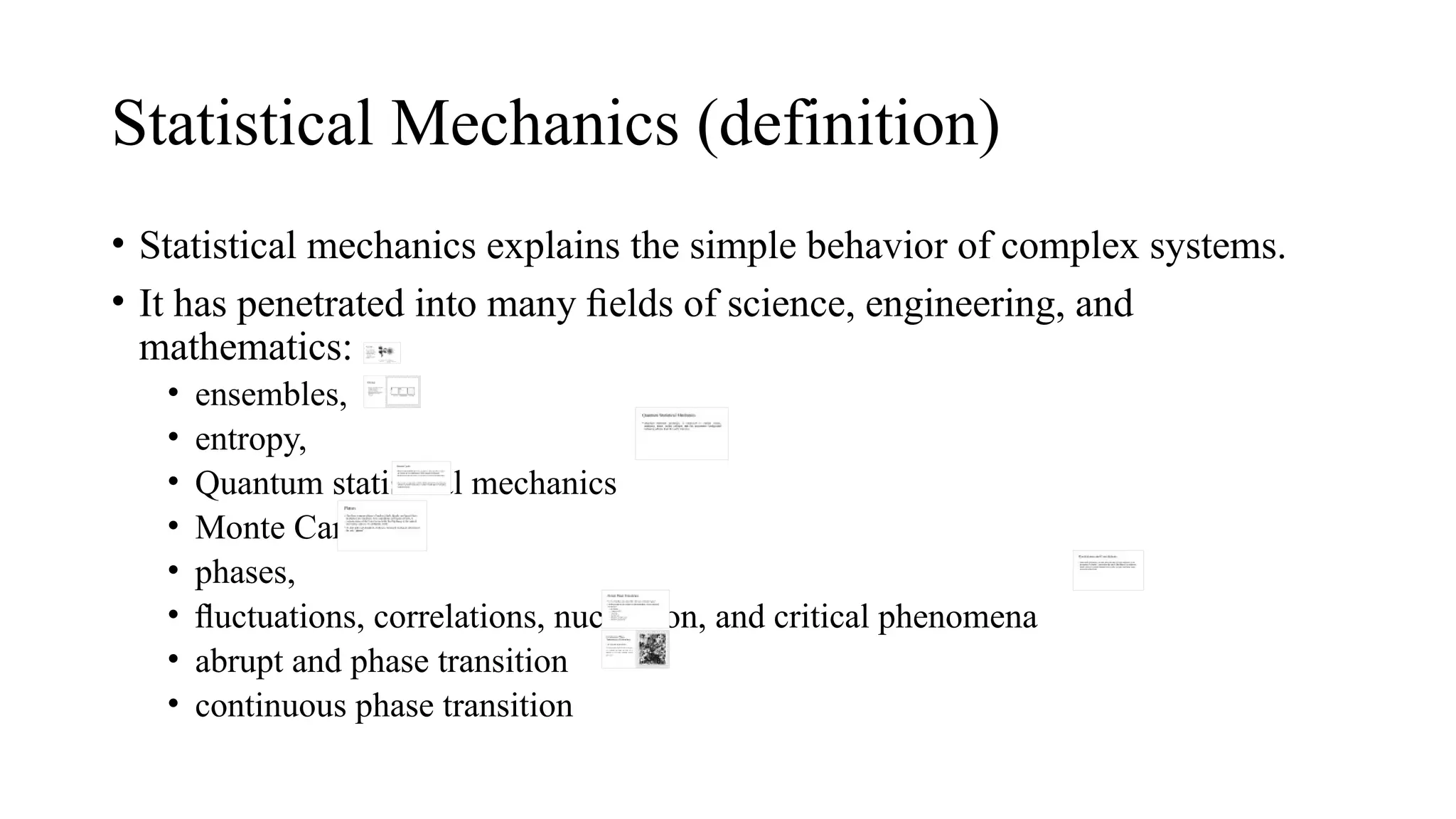
• Statistical mechanics explains the simple behavior of complex systems.
• It has penetrated into many ﬁelds of science, engineering, and
mathematics:
• ensembles,
• entropy,
• Quantum statistical mechanics
• Monte Carlo,
• phases,
• ﬂuctuations, correlations, nucleation, and critical phenomena
• abrupt and phase transition
• continuous phase transition

Ensembles
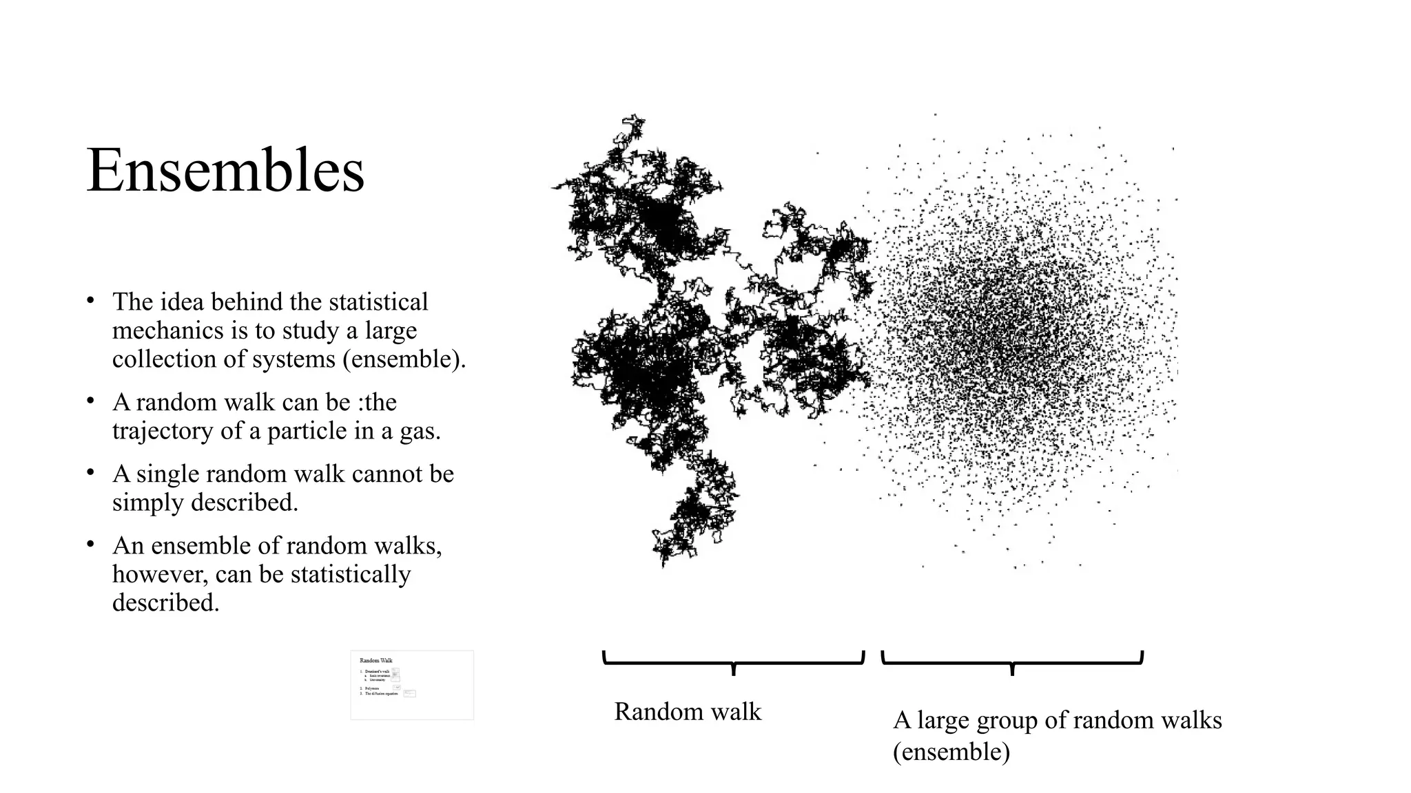
• The idea behind the statistical
mechanics is to study a large
collection of systems (ensemble).
• A random walk can be :the
trajectory of a particle in a gas.
• A single random walk cannot be
simply described.
• An ensemble of random walks,
however, can be statistically
described.
Random walk A large group of random walks
(ensemble)

Entropy
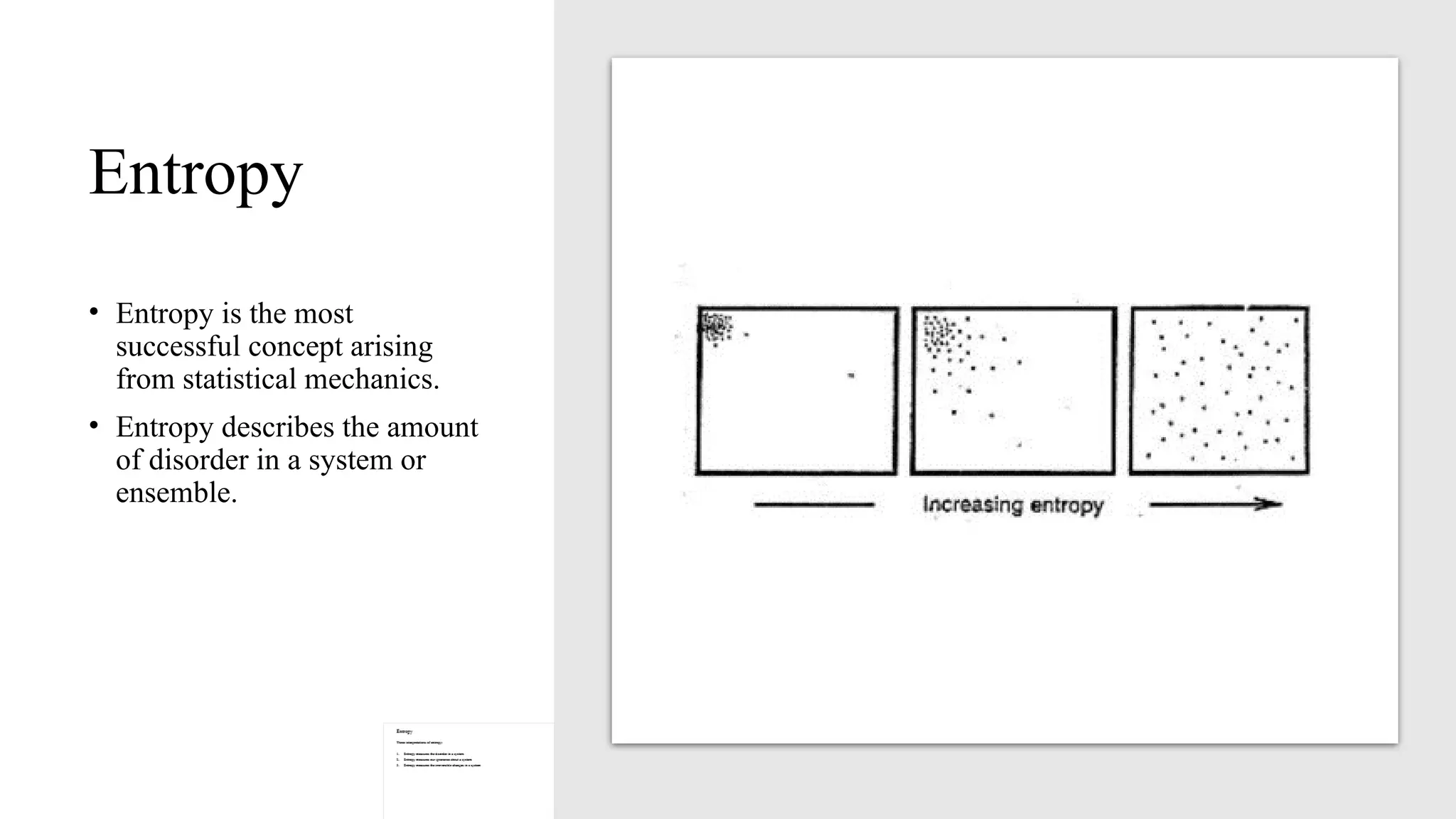
• Entropy is the most
successful concept arising
from statistical mechanics.
• Entropy describes the amount
of disorder in a system or
ensemble.

Quantum Statistical Mechanics
• Quantum statistical mechanics is employed to explain metals,
insulators, lasers, stellar collapse, and the microwave background
radiation patterns from the early Universe.

Monte Carlo
• Monte Carlo methods allow the computer to find ensemble averages
in systems far too complicated to allow analytical evaluation.
• Monte Carlo tools are used in everywhere in science and technology.
• These tools are applicable in diverse fields starting from simulating
the interiors of particle accelerators, to studies of tra c flow, to
ffi
designing computer circuits.

Phases
• The three common phases of matter (solids, liquids, and gases) have
multiplied into hundreds: from superﬂuids and liquid crystals, to
vacuum states of the Universe just after the Big Bang, to the pinned
and sliding ‘phases’ of earthquake faults.
• To deal with such hundreds of phases, statistical mechanics introduced
the tool “phases”.

Fluctuations and Correlations
• Statistical mechanics not only describes the average behavior of an
ensemble of systems, it describes the entire distribution of behaviors
based on how systems ﬂuctuate and evolve in space and time using
correlation functions.

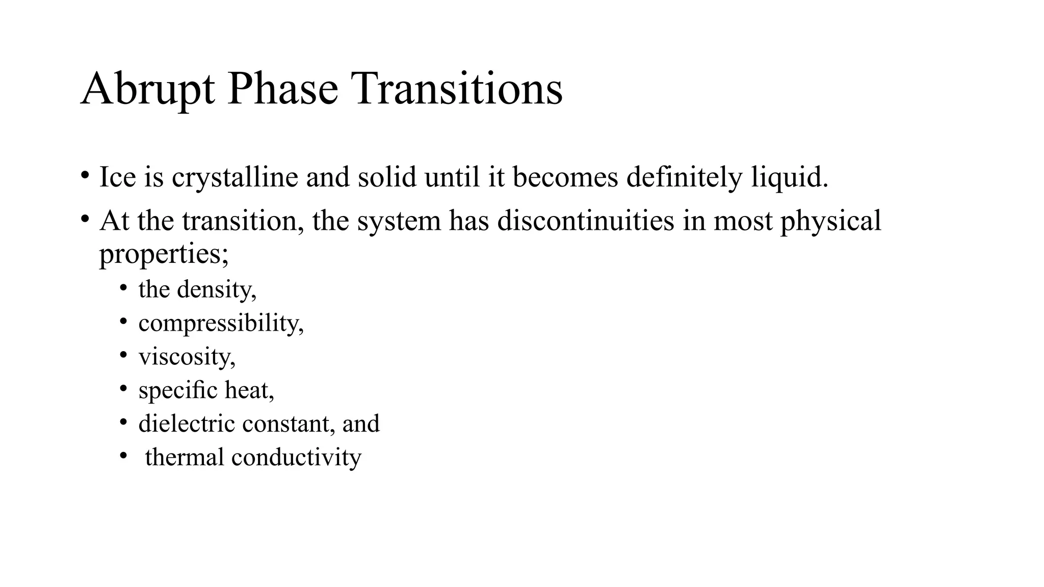
Abrupt Phase Transitions
• Ice is crystalline and solid until it becomes definitely liquid.
• At the transition, the system has discontinuities in most physical
properties;
• the density,
• compressibility,
• viscosity,
• speciﬁc heat,
• dielectric constant, and
• thermal conductivity

Continuous Phase
Transitions (Criticality)
• The self-similar, fractal structures;
The system cannot decide whether to stay
gray or to separate into black and white, so it
ﬂuctuates on all scales, exhibiting critical
phenomena.

Random Walk
1. Drunkard’s walk
a. Scale invariance
b. Universality
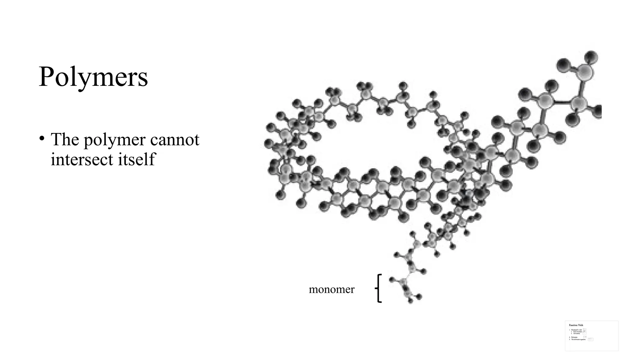
2. Polymers
3. The di usion equation
ﬀ

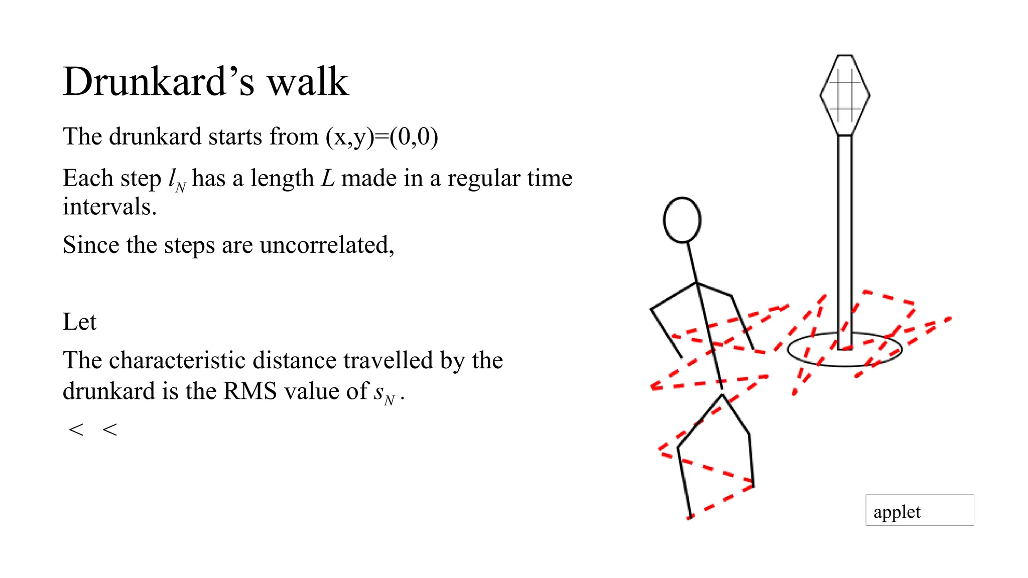
Drunkard’s walk
The drunkard starts from (x,y)=(0,0)
Each step lN has a length L made in a regular time
intervals.
Since the steps are uncorrelated,
Let
The characteristic distance travelled by the
drunkard is the RMS value of sN .
< <
applet

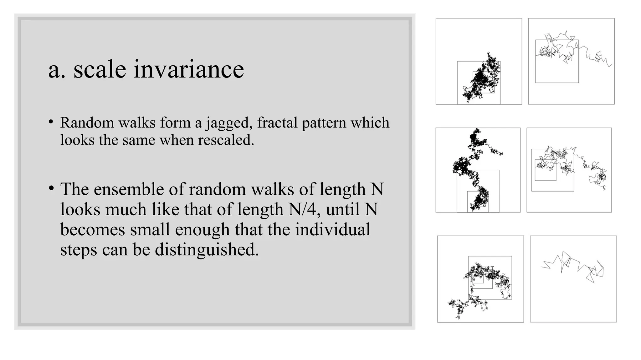
a. scale invariance
• Random walks form a jagged, fractal pattern which
looks the same when rescaled.
• The ensemble of random walks of length N
looks much like that of length N/4, until N
becomes small enough that the individual
steps can be distinguished.

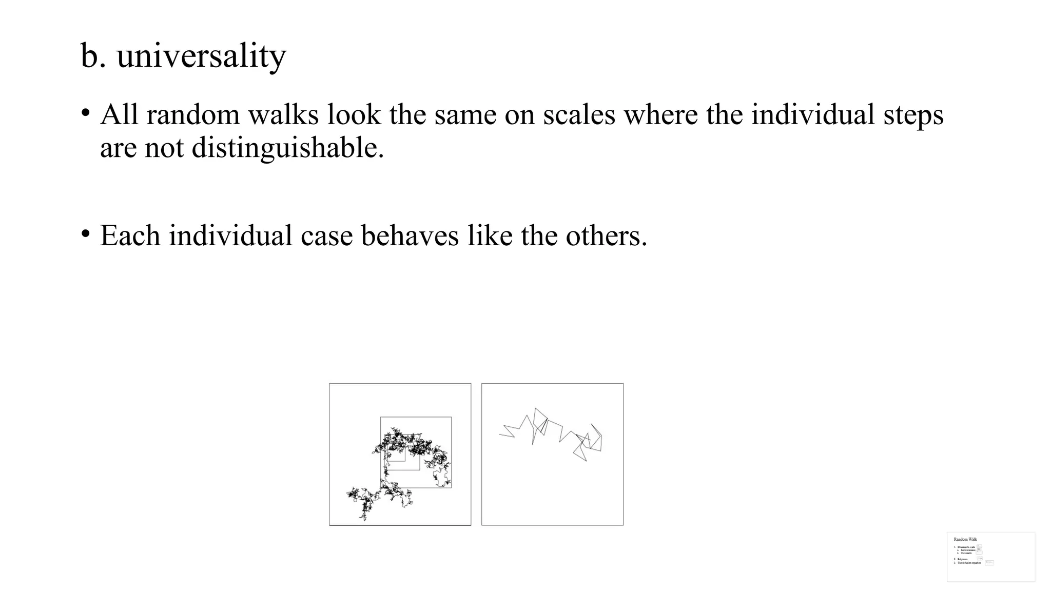
b. universality
• All random walks look the same on scales where the individual steps
are not distinguishable.
• Each individual case behaves like the others.

Polymers
• The polymer cannot
intersect itself
monomer

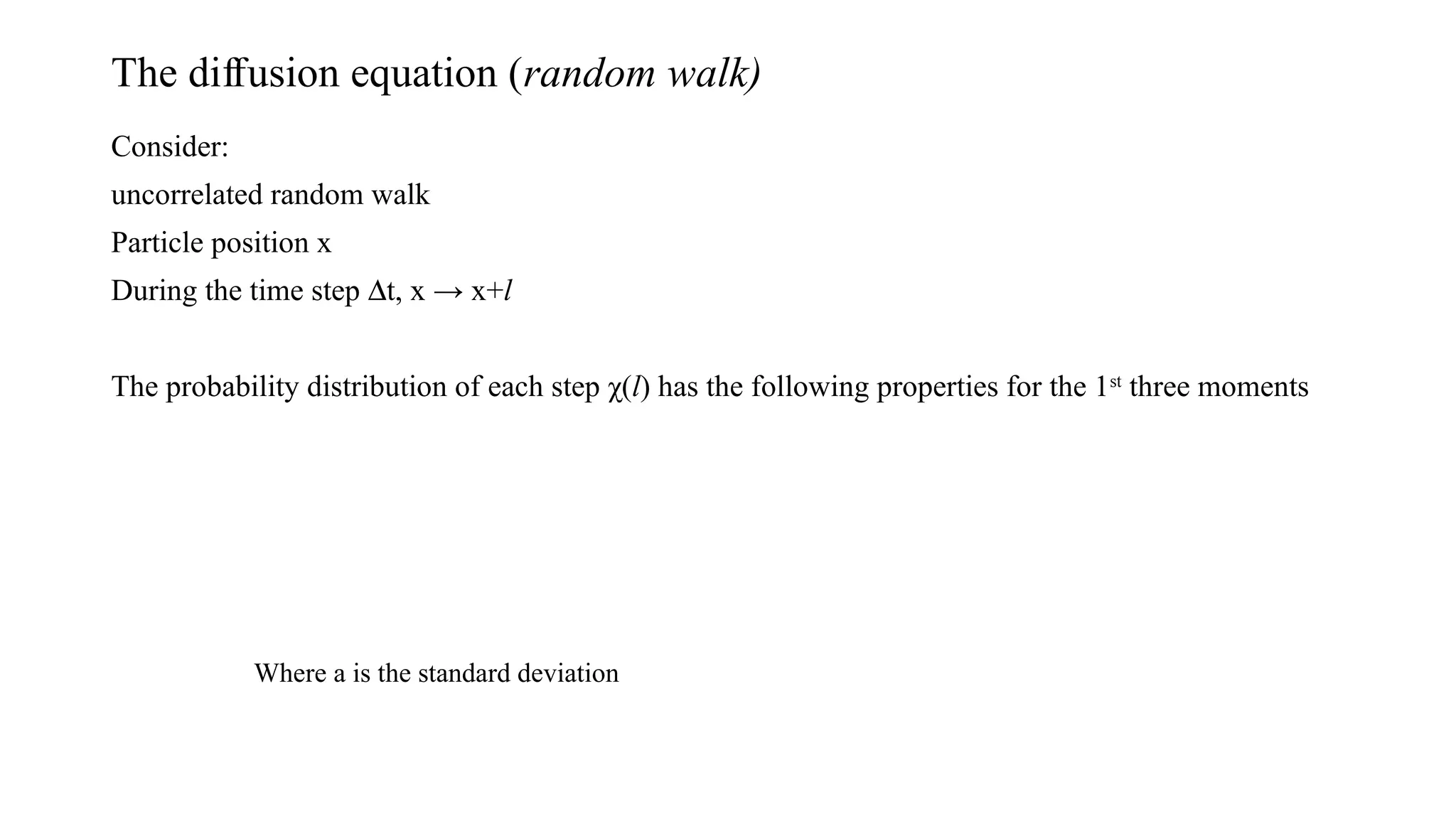
The di usion equation (
ﬀ random walk)
Consider:
uncorrelated random walk
Particle position x
During the time step Dt, x → x+l
The probability distribution of each step χ(l) has the following properties for the 1st
three moments
Where a is the standard deviation

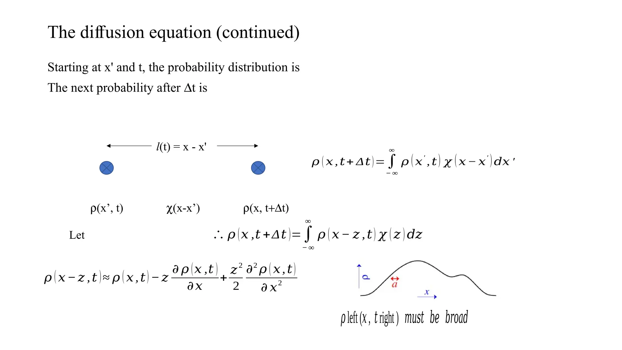
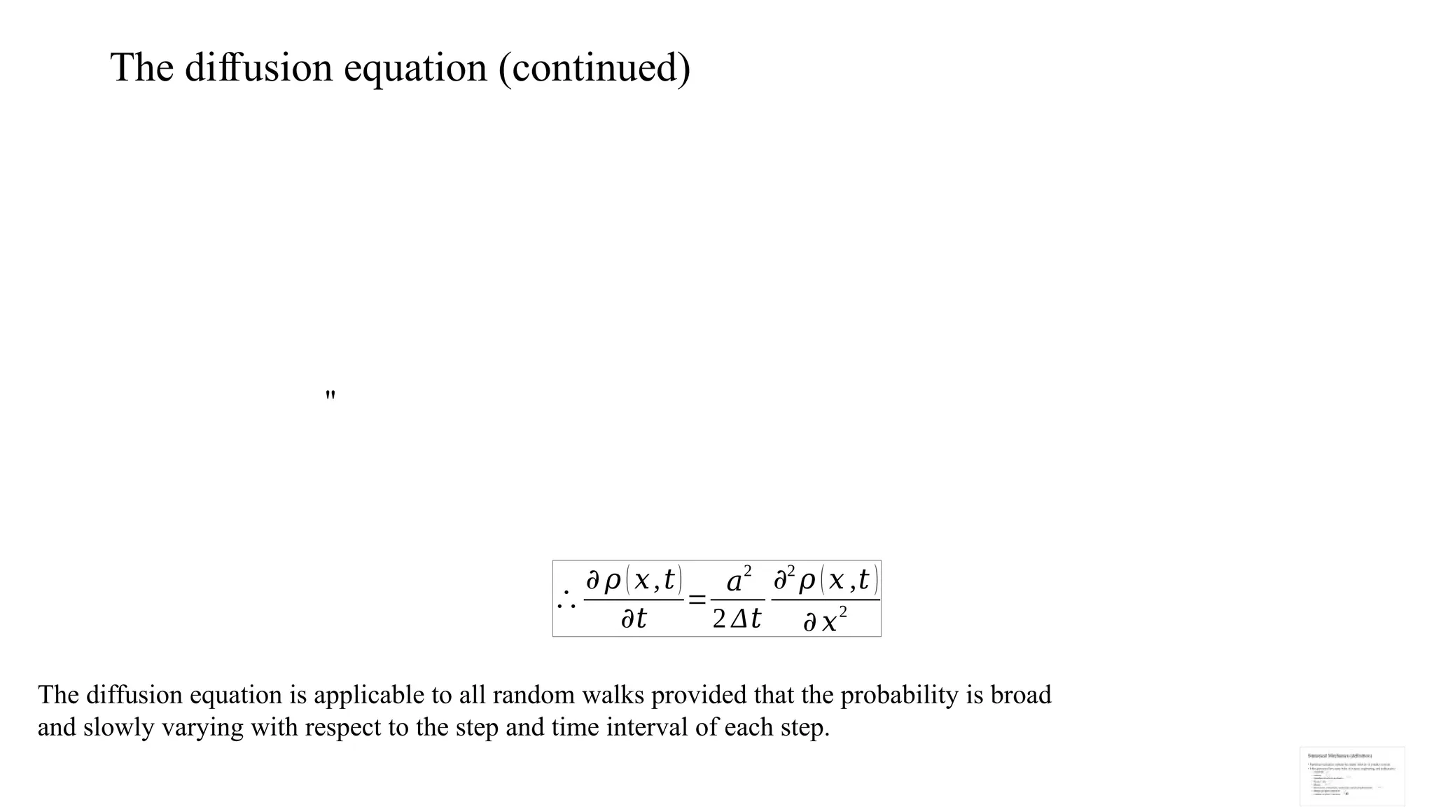
The di usion equation (continued)
ﬀ
Starting at x' and t, the probability distribution is
The next probability after Dt is
r(x’, t) r(x, t+Dt)
l(t) = x - x'
c(x-x’)
𝜌 ( 𝑥 , 𝑡+ Δ𝑡)=∫
− ∞
∞
𝜌 (𝑥
′
, 𝑡) 𝜒 (𝑥 − 𝑥
′
)𝑑𝑥 ′
Let ∴ 𝜌 (𝑥 ,𝑡 +Δ𝑡 )=∫
− ∞
∞
𝜌 (𝑥− 𝑧 ,𝑡) 𝜒 ( 𝑧 )𝑑𝑧
𝜌 (𝑥−𝑧 ,𝑡 )≈ 𝜌 ( 𝑥,𝑡) − 𝑧
𝜕 𝜌 (𝑥 ,𝑡 )
𝜕𝑥
+
𝑧2
2
𝜕2
𝜌 ( 𝑥,𝑡)
𝜕 𝑥2
left( , right)
𝜌 𝑥 𝑡 𝑚𝑢𝑠𝑡 𝑏𝑒 𝑏𝑟𝑜𝑎𝑑

The di usion equation (continued)
ﬀ
"
∴
𝜕 𝜌 (𝑥,𝑡)
𝜕𝑡
=
𝑎
2
2 Δ𝑡
𝜕2
𝜌 (𝑥 ,𝑡 )
𝜕 𝑥2
The diffusion equation is applicable to all random walks provided that the probability is broad
and slowly varying with respect to the step and time interval of each step.

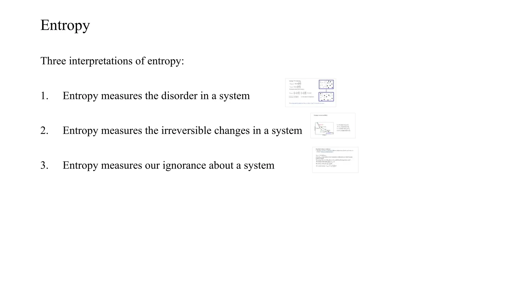
Entropy
Three interpretations of entropy:
1. Entropy measures the disorder in a system
2. Entropy measures the irreversible changes in a system
3. Entropy measures our ignorance about a system

Entropy "S" of mixing
The change in entropy due to mixing is
N/2 N/2
N
𝑆𝑐𝑜𝑢𝑛𝑡𝑖𝑛𝑔=𝑘𝐵 log [𝑚] m is the number of configurations
The entropy gains kB log(m) each time we add an “atom” to one of the two boxes

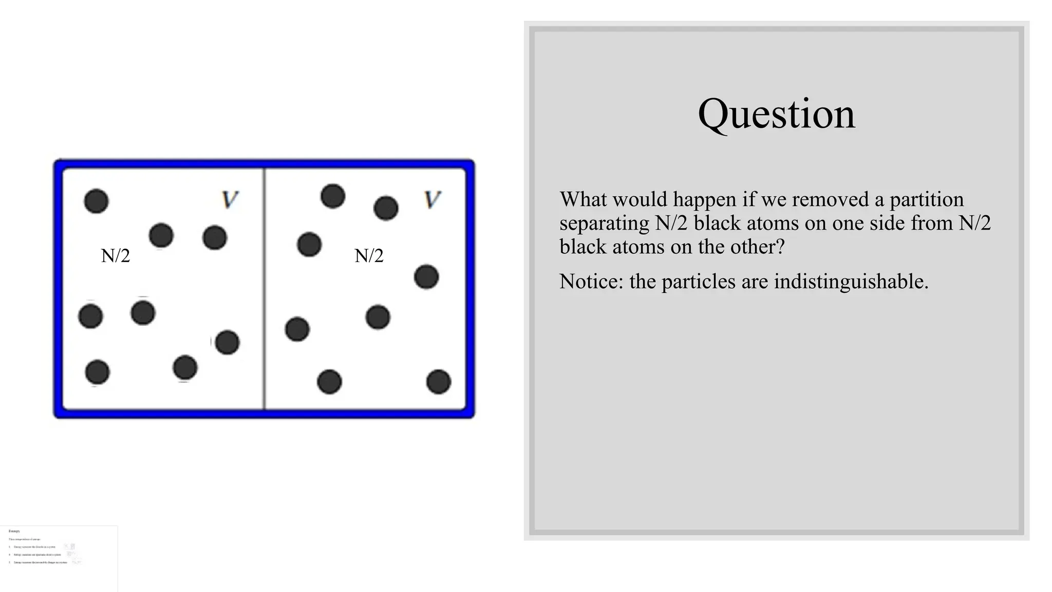
Question
What would happen if we removed a partition
separating N/2 black atoms on one side from N/2
black atoms on the other?
Notice: the particles are indistinguishable.
N/2 N/2

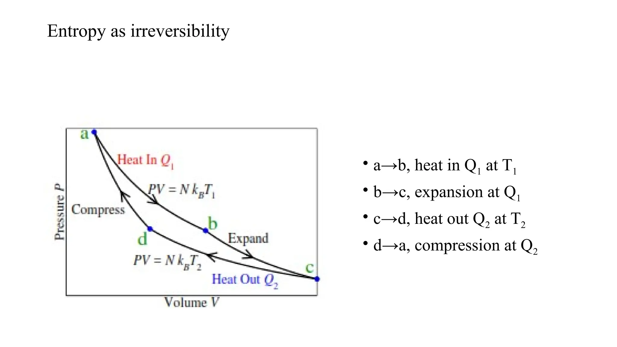
Entropy as irreversibility
• a→b, heat in Q1 at T1
• b→c, expansion at Q1
• c→d, heat out Q2 at T2
• d→a, compression at Q2

The ideal gas equation
For the ideal gas, the total energy E = kinetic energy,
Energy conservation (regions a to b, c to d) requires that

In case of expansion (b to c) and compression (d to a):
Conservation of energy requires:

Residual entropy of glasses
• The glass will have a completely di erent conﬁguration of atoms each time it is
ﬀ
formed. "it has a residual entropy"
where,Ωglass is the number of zero temperature configurations in which the glass
might be trapped.
The entropy flow out of the glass as it is cooled from the liquid state is Q/T
The entropy of the liquid 'glass' Sliquid (Tl)
The entropy of the glass
The residual entropy= Sliquid (Tl)-

Non-equilibrium entropy (Discrete)
• Probability distribution among a discrete set of states
The entropy of M equally likely states is
The probability of each state is
If ri is not constant
Out of equilibrium system

Non-equilibrium entropy (continuum)
•
• =

Quantum statistical mechanics
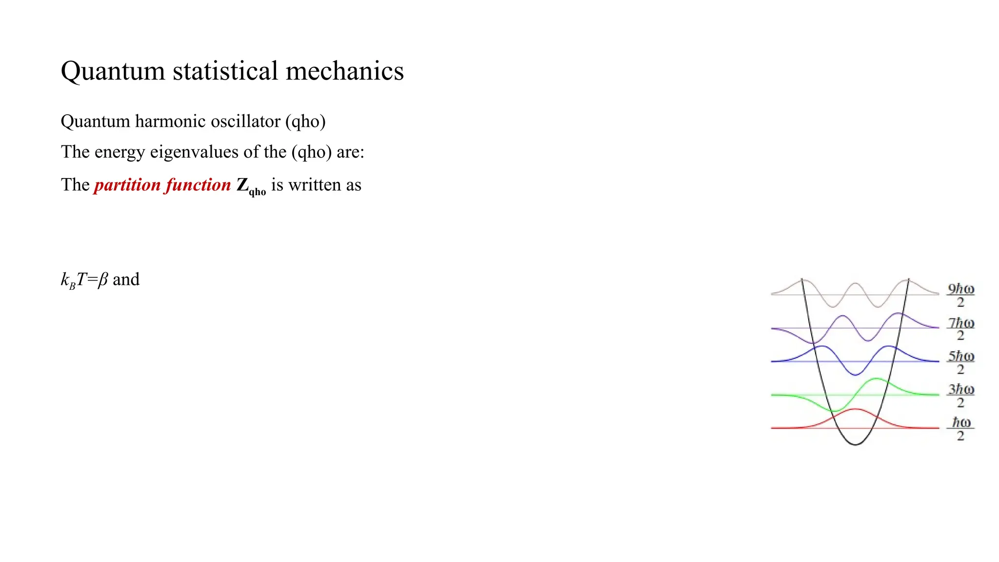
Quantum harmonic oscillator (qho)
The energy eigenvalues of the (qho) are:
The partition function Zqho is written as
kBT=β and

Average energy and the average excitation level
Since and
Compare (1) and (2),
The average excitation level
Specific heat cv is

Classical specific heat
Quantum statistical mechanics describes classical states as well.
according to equation (3), and at high T, cV approaches kB, a constant
value.
At very low temperature, T goes to 0, there still an energy of the
harmonic oscillator, .
Classically, at T=0 there is no oscillations.

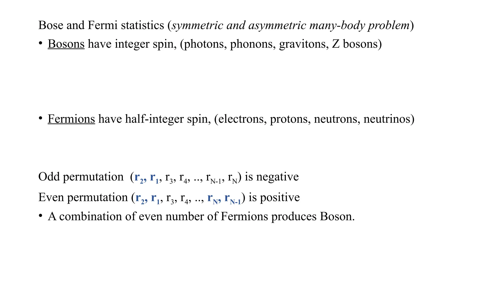
Bose and Fermi statistics (symmetric and asymmetric many-body problem)
• Bosons have integer spin, (photons, phonons, gravitons, Z bosons)
• Fermions have half-integer spin, (electrons, protons, neutrons, neutrinos)
Odd permutation (r2, r1, r3, r4, .., rN-1, rN) is negative
Even permutation (r2, r1, r3, r4, .., rN, rN-1) is positive
• A combination of even number of Fermions produces Boson.

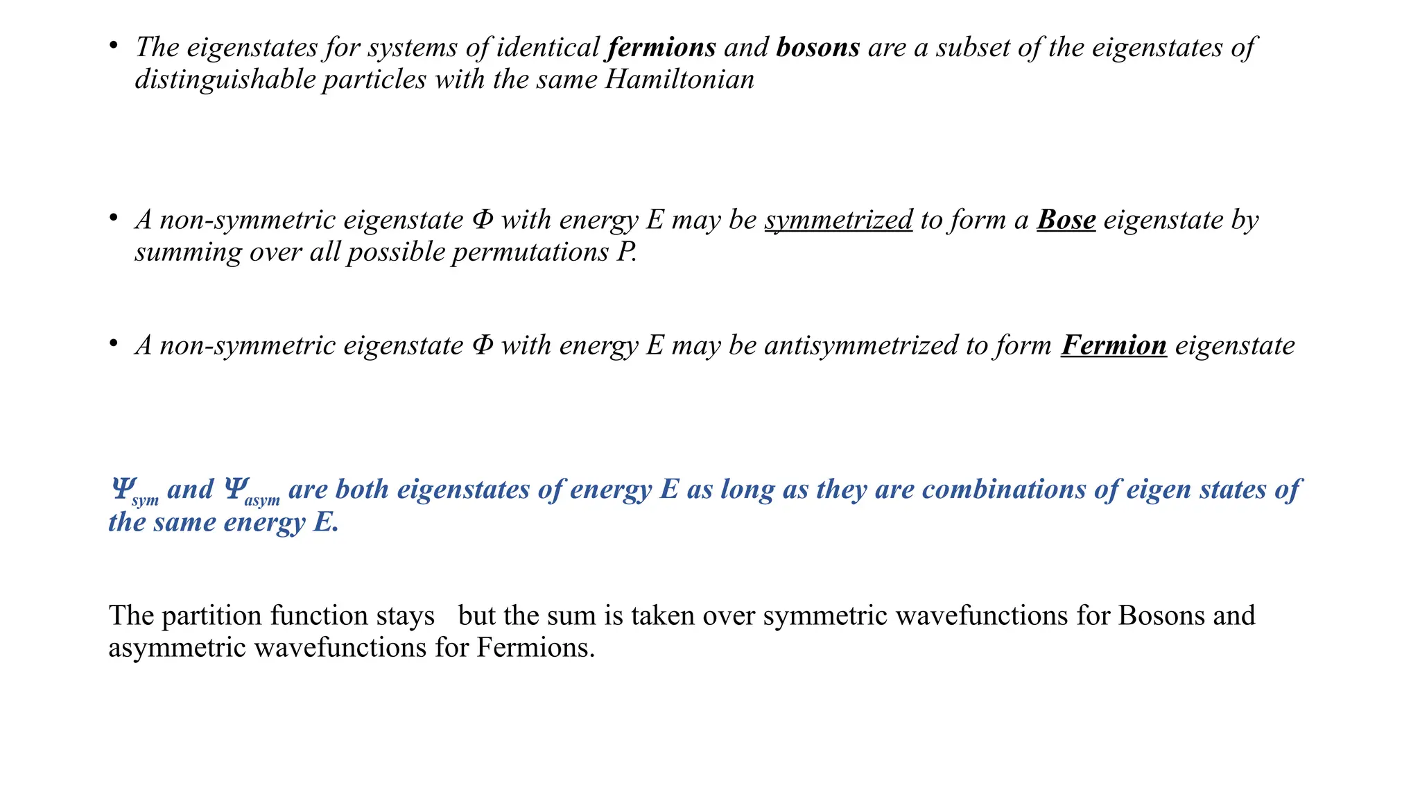
• The eigenstates for systems of identical fermions and bosons are a subset of the eigenstates of
distinguishable particles with the same Hamiltonian
• A non-symmetric eigenstate Φ with energy E may be symmetrized to form a Bose eigenstate by
summing over all possible permutations P.
• A non-symmetric eigenstate Φ with energy E may be antisymmetrized to form Fermion eigenstate
Ysym and Yasym are both eigenstates of energy E as long as they are combinations of eigen states of
the same energy E.
The partition function stays but the sum is taken over symmetric wavefunctions for Bosons and
asymmetric wavefunctions for Fermions.

Non-interacting many-body problem (Bosons and Fermions)
is the jth
particle Hamiltonian.
Where yk is the single particle eigenstate of the Hamiltonian H.
The many-body eigenstates are

Non-interacting Bosons
Symmetrizing over the coordinates rj:

Antisymmetrizing over all N! possible permutations
Non-interacting Fermions

Pauli exclusion principle
Two different eigenstates:
Distinguishable particles:
Bosons:
Fermions:
If the two Fermions "are" in the same eigenstate ,
No two Fermions can occupy the same quantum eigenstate.

Advanced statistics are the mathematical tools used to discover and explore complex relationships between different variables in large datasets.

More Related Content

Similar to Advanced statistics are the mathematical tools used to discover and explore complex relationships between different variables in large datasets.

Recently uploaded

Advanced statistics are the mathematical tools used to discover and explore complex relationships between different variables in large datasets.